
Larger than memory datasets#
Modern health datasets can become very large. When datasets are so large they cannot be loaded into a computer’s memory at once and loading & processing the data in batches becomes necessary (“out-of-core”).
Dask is a popular out-of-core, distributed array processing library that ehrapy is beginning to support.
Here we show how dask support in ehrapy can reduce the memory consumption of a simple ehrapy processing workflow.
🔪 Beware sharp edges! 🔪
dask support in ehrapy is new and highly experimental!
Many functions in ehrapy do not support dask and may exhibit unexpected behaviour if dask arrays are passed to them.
Stick to what’s outlined in this tutorial and you should be fine!
Example Usecase#
We can now profile the required time and memory consumption of two runs for processing this data:
In memory (which is feasible with our demo dataset)
Out-of-core
We will compare these two on a synthetic dataset of 50’000 samples and 1’000 features, with 4 distinct groups underlying the data generation process.
On this dataset, we
Scale the data to zero mean and unit variance
Compute a PCA
Compute a neighborhood graph on PCA space
Perform clustering in the neighborhood graph
Project the data to the top two Principal Components space, and color the found clusters for visualization.
Profiled Code#
Memory#
For the in-memory setting, the following code is used to generate profiling results:
import scalene

scalene.scalene_profiler.stop()

import pandas as pd
from sklearn.datasets import make_blobs as make_blobs
import ehrapy as ep
import ehrdata as ed

n_individuals = 50000
n_features = 1000
n_groups = 4
chunks = 1000

data_features, data_labels = make_blobs(
    n_samples=n_individuals, n_features=n_features, centers=n_groups, random_state=42
)

var = pd.DataFrame({"feature_type": ["numeric"] * n_features})

edata = ed.EHRData(X=data_features, obs={"label": data_labels}, var=var)

scalene.scalene_profiler.start()

ep.pp.scale_norm(edata)

ep.pp.pca(edata)

ep.pp.neighbors(edata)

ep.tl.leiden(edata)

ep.pl.pca(edata, color="leiden", save="profiling_memory_pca.png")

scalene.scalene_profiler.stop()
Out-of-core#
For the out-of-core setting, the following code is used to generate profiling results:
import scalene

scalene.scalene_profiler.stop()

import dask.array as da
from sklearn.datasets import make_blobs as make_blobs
import ehrapy as ep
import pandas as pd

n_individuals = 50000
n_features = 1000
n_groups = 4
chunks = 1000

data_features, data_labels = make_blobs(
    n_samples=n_individuals, n_features=n_features, centers=n_groups, random_state=42
)

data_features = da.from_array(data_features, chunks=chunks)

var = pd.DataFrame({"feature_type": ["numeric"] * n_features})

edata = ed.EHRData(X=data_features, obs={"label": data_labels}, var=var)

scalene.scalene_profiler.start()

ep.pp.scale_norm(edata)

ep.pp.pca(edata)

edata.obsm["X_pca"] = edata.obsm["X_pca"].compute()

ep.pp.neighbors(edata)

ep.tl.leiden(edata)

ep.pl.pca(edata, color="leiden", save="profiling_out_of_core_pca.png")

scalene.scalene_profiler.stop()
Optional: Try it Yourself#
Click here for instructions of how to run the profiling results yourself.
Workflow:
Setup
The results shown in this notebook rely on optional dependencies of ehrapy. Also, we will use scalene for profiling. You can install these required tools into your environment with:
pip install ehrapy[dask] scalene
Profile runs
Scalene currently requires code to be run as Python script for a full profile. For this, copy the above code snippets into two Python files “profile_memory.py” and “profile_out_of_core.py”, respectively.
Then, from your commmand line within this environment run
scalene profile_memory.py --outfile profile_memory.html
for the in-memory computation and
scalene profile_out_of_core.py --outfile profile_out_of_core.html
for the out-of-core computation.
Setup The results shown in this notebook rely on optional dependencies of
ehrapy. Also, we will use scalene for profiling. You can install these required tools into your environment with:
pip install ehrapy[dask] scalene
Profile runs Scalene currently requires code to be run as Python script for a full profile. For this, copy the above code snippets into two Python files “profile_memory.py” and “profile_out_of_core.py”, respectively. Then, from your commmand line within this environment run
scalene profile_memory.py --outfile profile_memory.html
for the in-memory computation and
scalene profile_out_of_core.py --outfile profile_out_of_core.html
for the out-of-core computation.
Results#
The resulting Scalene profiles can depend on the machine and environment the profiling is run. Here, we show results obtained on an Intel(R) Core(TM) i7-8565U CPU @ 1.80GHz laptop.
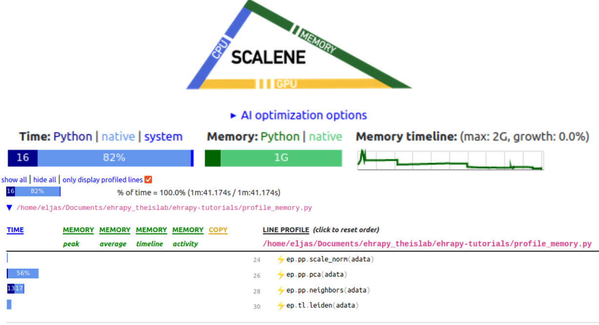
In Memory Profile#
Out-of-core Profile#

There are multiple features in scalene’s output, we show and focus on the key aspects here.
Time#
The required time for the profiled code to execute is displayed at the topmost “% of time = 100.0%”. We can see that for the in-memory computation, the required wall time was 1 min 41 seconds, whereas for the out-of-core computation, the required wall time was 1 min 39 seconds.
Generally, the out-of-core computation can yield performance improvements by optimizing the scheduling of computations by using “lazy execution”, for which you can find more information here. Dask also allows distributed computations, providing even further speed improvements.
Beware that especially for small dataset or small chunk sizes, the overhead of such out-of-core computations can also exceed the gains obtained.
Here, we can see that the order of magnitude for execution time for both workflows is similar.
Maximum Memory Consumption#
The maximum required memory for the profiled code is displayed at the top right, on top of the “Memory timeline” plot. We can see that the maximum memory occupation for the in-memory computation was 2 GB, whereas for the out-of-core computation, the maximum memory occupation was 193 MB.
This can be achieved by leveraging the key idea behind dask, its block-wise (“chunked”) computations. This means that dask accesses the data in chunks, not requiring the entire dataset to be loaded to memory at once.
The size of the blocks is a tradeoff of having not too many small blocks (causing too much overhead) and not too big blocks (causing increased memory consumption and potentially less distributed computations). See here for a more detailed discussion on the block size.
Conclusion#
Here, we show with a synthetic dataset how out-of-core computations can reduce the memory requirements for a suite of analysis steps.
The dataset we have generated is small enough to not require out-of-core computations, so we can compare the in-memory and the out-of-core computation profiles.
In general, in-memory computations are to be preferred whenever they are feasible, being easier to perform and omit potential pitfals such as using too small chunk sizes.
We have computed a PCA and can observe that the four underlying groups in our synthetic data form well separated clusters in the two-dimensional PCA projection, and are well clustered by Leiden clustering.

Further support for dask is a work in progress. However, many operations past this point can work with the dimensionality reduction directly in memory.