
MIMIC-II IAC Survival Analysis#
This tutorial investigates survival of patients recorded in the MIMIC-II IAC dataset. It was created for the purpose of a case study to investigate the effectiveness of indwelling arterial catheters in hemodynamically stable patients with respiratory failure for mortality outcomes. This subset is derived from MIMIC-II, the publicly-accessible critical care database.
References:
[1] Critical Data, M.I.T., 2016. Secondary analysis of electronic health records (p. 427). Springer Nature. (https://link.springer.com/book/10.1007/978-3-319-43742-2)
[2] https://github.com/MIT-LCP/critical-data-book/tree/master/part_ii/chapter_16/jupyter
[3] https://stackoverflow.com/questions/27328623/anova-test-for-glm-in-python/60769343#60769343
More details on the dataset can be found here: https://physionet.org/content/mimic2-iaccd/1.0/.
Environment Setup#
import warnings

warnings.filterwarnings("ignore")

from itertools import product

import ehrapy as ep
import ehrdata as ed
import numpy as np
import pandas as pd
from statsmodels.stats.anova import anova_lm


MIMIC-II dataset preparation#
edata = ed.dt.mimic_2()
edata
EHRData object with n_obs × n_vars × n_t = 1776 × 46 × 1
    shape of .X: (1776, 46)
The MIMIC-II dataset has 1776 patients as described above with 46 features.
Linear Regression#
Introduction#
Linear regression provides the foundation for many types of analyses we perform on health data. In the simplest scenario, we try to relate one continuous outcome, \(y\), to a single continuous covariate, \(x\), by trying to find values for \(\beta_0\) and \(\beta_1\) so that the following equation describes our observations: \(y=\beta_0 + \beta_1 \times x\)
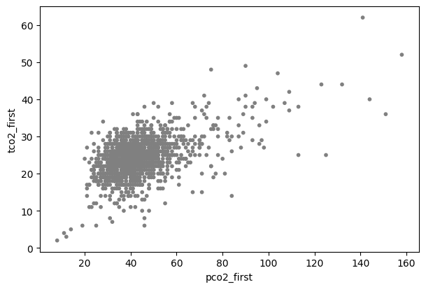
We examine whether the measurements are correlated:
ax = ep.pl.scatter(edata, x="pco2_first", y="tco2_first")
var_names = ["pco2_first", "tco2_first", "gender_num"]
formula = "tco2_first ~ pco2_first"
co2_lm = ep.tl.ols(edata, var_names, formula, missing="drop")
Dissecting this command from left to right: The co2_lm = part assigns the right part of the command to a new variable called co2_lm.
The right side of this command runs the :func:ehrapy.tools.ols function.
Here, our outcome variable is called tco2_first and we are just fitting one covariate, pco2_first, so we define the formula as tco2_first ~ pco2_first.
The overall procedure of specifying a model formula (tco2_first ~ pco2_first), a data object (edata) and passing it an appropriate Python function (ep.tl.ols) will be used throughout these examples, and is the foundation for many types of statistical modeling in ehrapy.
Run the summary command for more model information.
co2_lm_result = co2_lm.fit()
co2_lm_result.summary()
| Dep. Variable: | tco2_first | R-squared: | 0.265 |
|---|---|---|---|
| Model: | OLS | Adj. R-squared: | 0.264 |
| Method: | Least Squares | F-statistic: | 571.8 |
| Date: | Fri, 27 Mar 2026 | Prob (F-statistic): | 3.52e-108 |
| Time: | 16:20:46 | Log-Likelihood: | -4609.1 |
| No. Observations: | 1590 | AIC: | 9222. |
| Df Residuals: | 1588 | BIC: | 9233. |
| Df Model: | 1 | ||
| Covariance Type: | nonrobust |
| coef | std err | t | P>|t| | [0.025 | 0.975] | |
|---|---|---|---|---|---|---|
| Intercept | 16.2109 | 0.360 | 45.071 | 0.000 | 15.505 | 16.916 |
| pco2_first | 0.1886 | 0.008 | 23.912 | 0.000 | 0.173 | 0.204 |
| Omnibus: | 94.233 | Durbin-Watson: | 1.963 |
|---|---|---|---|
| Prob(Omnibus): | 0.000 | Jarque-Bera (JB): | 195.722 |
| Skew: | -0.389 | Prob(JB): | 3.16e-43 |
| Kurtosis: | 4.532 | Cond. No. | 149. |
Notes:
[1] Standard Errors assume that the covariance matrix of the errors is correctly specified.
The best fit equation for the data as shown therefore is:
tco2_first = 16.21 + 0.189 \(\times\) pco2_first.
Model Selection#
We will begin by examining if the relationship between TCO2 and PCO2 is more complicated than the model we fit in the previous section.
If you recall, we fit a model where we considered a linear pco2_first term: tco2_first = \(\beta_0 + \beta_1 \times\) pco2_first.
One may wonder if including a quadratic term would fit the data better, i.e. whether:
tco2_first = \(\beta_0 + \beta_1 \times\) pco2_first + \(\beta_2 \times\) pco2_first\(^2\),
is a better model.
Adding a quadratic term (or any other function) is quite easy using :func:ehrapy.tools.ols.
Fitting this model, and running the summary function for the model:
formula = "tco2_first ~ pco2_first + np.square(pco2_first)"

o2_quad_lm = ep.tl.ols(edata, var_names, formula, missing="drop")
co2_quad_lm_result = o2_quad_lm.fit()
co2_quad_lm_result.summary()
| Dep. Variable: | tco2_first | R-squared: | 0.265 |
|---|---|---|---|
| Model: | OLS | Adj. R-squared: | 0.264 |
| Method: | Least Squares | F-statistic: | 285.7 |
| Date: | Fri, 27 Mar 2026 | Prob (F-statistic): | 1.04e-106 |
| Time: | 16:20:46 | Log-Likelihood: | -4609.1 |
| No. Observations: | 1590 | AIC: | 9224. |
| Df Residuals: | 1587 | BIC: | 9240. |
| Df Model: | 2 | ||
| Covariance Type: | nonrobust |
| coef | std err | t | P>|t| | [0.025 | 0.975] | |
|---|---|---|---|---|---|---|
| Intercept | 16.0916 | 0.771 | 20.862 | 0.000 | 14.579 | 17.605 |
| pco2_first | 0.1930 | 0.027 | 7.231 | 0.000 | 0.141 | 0.245 |
| np.square(pco2_first) | -3.569e-05 | 0.000 | -0.175 | 0.861 | -0.000 | 0.000 |
| Omnibus: | 93.522 | Durbin-Watson: | 1.963 |
|---|---|---|---|
| Prob(Omnibus): | 0.000 | Jarque-Bera (JB): | 194.937 |
| Skew: | -0.385 | Prob(JB): | 4.68e-43 |
| Kurtosis: | 4.533 | Cond. No. | 1.94e+04 |
Notes:
[1] Standard Errors assume that the covariance matrix of the errors is correctly specified.
[2] The condition number is large, 1.94e+04. This might indicate that there are
strong multicollinearity or other numerical problems.
Looking first at the coefficients estimates, we see the best fit line is estimated as:
tco2_first = 16.09 + 0.19 \(\times\) pco2_first + 0.00004 \(\times\) pco2_first\(^2\).
We can add both best fit lines to the former scattered points using the :func:ehrapy.plot.ols function:
ep.pl.ols(
    edata,
    x="pco2_first",
    y="tco2_first",
    ols_results=[co2_lm_result, co2_quad_lm_result],
    ols_color=["red", "blue"],
    xlabel="PCO2",
    ylabel="TCO2",
)
Figure Scatterplot of PCO2 (x-axis) and TCO2 (y-axis) along with linear regression estimates from the quadratic model (co2_quad_lm) and linear only model (co2_lm)
The red (linear term only) and blue (linear and quadratic terms) fits are nearly identical.
This corresponds with the relatively small coefficient estimate for the (pco2_first^2) term.
The p-value for this coefficient is about 0.86, and at the 0.05 significance level we would likely conclude that a quadratic term is not necessary in our model to fit the data, as the linear term only model fits the data nearly as well.
Statistical Interactions and Testing Nested Models#
We can also consider additional features in our model.
For this, we can start with e.g. gender as a covariate, but no interaction.
We can do this by simply adding the variable gender_num to the previous formula for our co2_lm model fit.
formula = "tco2_first ~ pco2_first + gender_num"
var_names = ["tco2_first", "pco2_first", "gender_num"]
co2_gender_lm = ep.tl.ols(edata, var_names, formula, missing="drop")
co2_gender_lm_result = co2_gender_lm.fit()
co2_gender_lm_result.summary()
| Dep. Variable: | tco2_first | R-squared: | 0.265 |
|---|---|---|---|
| Model: | OLS | Adj. R-squared: | 0.264 |
| Method: | Least Squares | F-statistic: | 286.1 |
| Date: | Fri, 27 Mar 2026 | Prob (F-statistic): | 7.60e-107 |
| Time: | 16:20:46 | Log-Likelihood: | -4608.7 |
| No. Observations: | 1590 | AIC: | 9223. |
| Df Residuals: | 1587 | BIC: | 9240. |
| Df Model: | 2 | ||
| Covariance Type: | nonrobust |
| coef | std err | t | P>|t| | [0.025 | 0.975] | |
|---|---|---|---|---|---|---|
| Intercept | 16.3044 | 0.378 | 43.166 | 0.000 | 15.564 | 17.045 |
| pco2_first | 0.1889 | 0.008 | 23.922 | 0.000 | 0.173 | 0.204 |
| gender_num | -0.1817 | 0.224 | -0.812 | 0.417 | -0.621 | 0.257 |
| Omnibus: | 94.658 | Durbin-Watson: | 1.964 |
|---|---|---|---|
| Prob(Omnibus): | 0.000 | Jarque-Bera (JB): | 194.982 |
| Skew: | -0.394 | Prob(JB): | 4.57e-43 |
| Kurtosis: | 4.524 | Cond. No. | 160. |
Notes:
[1] Standard Errors assume that the covariance matrix of the errors is correctly specified.
This output is very similar to what we had before, but now there’s a gender_num term as well.
The 1 is present in the first column after gender_num, and it tells us who this coefficient is relevant to (subjects with 1 for the gender_num - men).
This is always relative to the baseline group, and in this case this is women.
The estimate is negative, meaning that the line fit for males will be below the line for females.
Plotting this fit curve:
# s stands for slope of the line, i stands for intercept of the line
s_female = co2_gender_lm_result.params[1]
i_female = co2_gender_lm_result.params[0]
s_male = co2_gender_lm_result.params[1]
i_male = co2_gender_lm_result.params[0] + co2_gender_lm_result.params[2]
ep.pl.ols(
    lines=[(s_female, i_female), (s_male, i_male)],
    lines_color=["k", "r"],
    lines_label=["Female", "Male"],
    xlabel="PCO2",
    ylabel="TCO2",
    xlim=(0, 40),
    ylim=(15, 25),
)
We see that the lines are parallel, but almost indistinguishable.
From the estimate from the summary output above, the difference between the two lines is -0.182 mmol/L, which is quite small, so perhaps this isn’t too surprising.
We can also see in the above summary output that the p-value is about 0.42, and we would likely not reject the null hypothesis that the true value of the gender_num coefficient is zero.
Next, we can explore our model with an interaction between pco2_first and gender_num.
To add an interaction between two variables use the * operator within a model formula.
By default, all of the main effects (variables contained in the interaction) are added to the model as well, so simply adding pco2_first*gender_num will add effects for pco2_first and gender_num in addition to the interaction between them to the model fit.
formula = "tco2_first ~ pco2_first * gender_num"
var_names = ["tco2_first", "pco2_first", "gender_num"]

co2_gender_interaction_lm = ep.tl.ols(edata, var_names, formula, missing="drop")
co2_gender_interaction_lm_result = co2_gender_interaction_lm.fit()
co2_gender_interaction_lm_result.summary()
| Dep. Variable: | tco2_first | R-squared: | 0.266 |
|---|---|---|---|
| Model: | OLS | Adj. R-squared: | 0.265 |
| Method: | Least Squares | F-statistic: | 191.6 |
| Date: | Fri, 27 Mar 2026 | Prob (F-statistic): | 5.09e-106 |
| Time: | 16:20:46 | Log-Likelihood: | -4607.7 |
| No. Observations: | 1590 | AIC: | 9223. |
| Df Residuals: | 1586 | BIC: | 9245. |
| Df Model: | 3 | ||
| Covariance Type: | nonrobust |
| coef | std err | t | P>|t| | [0.025 | 0.975] | |
|---|---|---|---|---|---|---|
| Intercept | 15.8544 | 0.489 | 32.443 | 0.000 | 14.896 | 16.813 |
| pco2_first | 0.1994 | 0.011 | 18.585 | 0.000 | 0.178 | 0.220 |
| gender_num | 0.8144 | 0.722 | 1.128 | 0.260 | -0.602 | 2.231 |
| pco2_first:gender_num | -0.0230 | 0.016 | -1.450 | 0.147 | -0.054 | 0.008 |
| Omnibus: | 97.108 | Durbin-Watson: | 1.964 |
|---|---|---|---|
| Prob(Omnibus): | 0.000 | Jarque-Bera (JB): | 200.324 |
| Skew: | -0.403 | Prob(JB): | 3.16e-44 |
| Kurtosis: | 4.541 | Cond. No. | 399. |
Notes:
[1] Standard Errors assume that the covariance matrix of the errors is correctly specified.
The estimated coefficients are \(\hat{\beta}_0, \hat{\beta}_1, \hat{\beta}_2\) and \(\hat{\beta}_3\), respectively, and we can determine the best fit lines for men:
tco2_first = \((15.85 + 0.81)\) + \((0.20 - 0.023)\) \(\times\) pco2_first = \(16.67\) + \(0.18\) \(\times\) pco2_first,
and for women:
tco2_first = \(15.85\) + \(0.20\) \(\times\) pco2_first.
Based on this, the men’s intercept should be higher, but their slope should be not as steep, relative to the women.
slope_female_interaction = co2_gender_interaction_lm_result.params[1]
intercept_female_interaction = co2_gender_interaction_lm_result.params[0]
slope_male_interaction = co2_gender_interaction_lm_result.params[1] + co2_gender_interaction_lm_result.params[3]
intercept_male_interaction = co2_gender_interaction_lm_result.params[0] + co2_gender_interaction_lm_result.params[2]

lines = [
    (s_female, i_female),
    (s_male, i_male),
    (slope_female_interaction, intercept_female_interaction),
    (slope_male_interaction, intercept_male_interaction),
]
lines_color = ["k", "r", "k", "r"]
lines_style = ["-", "-", ":", ":"]
lines_label = [
    "Female",
    "Male",
    "Female (Interaction Model)",
    "Male (Interaction Model)",
]
ep.pl.ols(
    lines=lines,
    lines_color=lines_color,
    lines_style=lines_style,
    lines_label=lines_label,
    xlabel="PCO2",
    ylabel="TCO2",
    xlim=(0, 40),
    ylim=(15, 25),
)
Regression fits of PCO2 on TCO2 with gender (black female; red male; solid no interaction; dotted with interaction). Note both axes are cropped for illustration purposes
We can see that the fits generated from this plot are a little different than the one generated for a model without the interaction.
The biggest difference is that the dotted lines are no longer parallel.
The estimated coefficient for the gender_num variable is now positive.
This means that at pco2_first=0, men (red) have higher tco2_first levels than women (black).
If you recall in the previous model fit, women had higher levels of tco2_first at all levels of pco2_first.
At some point around pco2_first=35 this changes and women (black) have higher tco2_first levels than men (red).
This means that the effect of gender_num may vary as you change the level of pco2_first, and is why interactions are often referred to as effect modification in the epidemiological literature.
The effect need not change signs (i.e., the lines do not need to cross) over the observed range of values for an interaction to be present.
The question remains, is the variable gender_num important?
We looked at this briefly when we examined the t value column in the no interaction model which included gender_num.
What if we wanted to test (simultaneously) the null hypothesis: \(\beta_2\) and \(\beta_3=0\).
The F-test can help us in this exact scenario where we want to look at if we should use a larger model (more covariates) or use a smaller model (fewer covariates).
The F-test applies only to nested models - the larger model must contain each covariate that is used in the smaller model, and the smaller model cannot contain covariates which are not in the larger model.
The interaction model and the model with gender are nested models since all the covariates in the model with gender are also in the larger interaction model.
An example of a non-nested model would be the quadratic model and the interaction model: the smaller (quadratic) model has a term (pco2_first\(^2\)) which is not in the larger (interaction) model.
An F-test would not be appropriate for this latter case.
To perform an F-test, first fit the two models you wish to consider, and then run the anova_lm command passing the two model objects.
anova_lm(co2_lm_result, co2_gender_interaction_lm_result)
| df_resid | ssr | df_diff | ss_diff | F | Pr(>F) | |
|---|---|---|---|---|---|---|
| 0 | 1588.0 | 30674.431382 | 0.0 | NaN | NaN | NaN |
| 1 | 1586.0 | 30621.082804 | 2.0 | 53.348578 | 1.381578 | 0.251484 |
The reported F-test p-value (Pr(>F)) in this case is 0.2515.
In nested models, the null hypothesis is that all coefficients in the larger model and not in the smaller model are zero.
In the case we are testing, our null hypothesis is \(\beta_2\) and \(\beta_3=0\).
Since the p-value exceeds the typically used significance level (\(\alpha=0.05\)), we would not reject the null hypothesis, and likely say the smaller model explains the data just as well as the larger model.
If these were the only models we were considering, we would use the smaller model as our final model and report the final model in our results.
We will now discuss what exactly to report and how to interpret the results.
Reporting and Interpreting Linear Regression#
Confidence and Prediction Intervals
As mentioned above, one method to quantify the uncertainty around coefficient estimates is by reporting the standard error. Another commonly used method is to report a confidence interval, most commonly a 95% confidence interval. A 95% confidence interval for \(\beta\) is an interval for which if the data were collected repeatedly, about 95% of the intervals would contain the true value of the parameter, \(\beta\), assuming the modeling assumptions are correct.
To get 95% confidence intervals of coefficients, The co2_lm_result has a function conf_int, which outputs 2.5% and 97.5% confidence interval limits for each coefficient.
print(co2_lm_result.conf_int())
                    0          1
Intercept   15.505369  16.916349
pco2_first   0.173103   0.204040
The 95% confidence interval for pco2_first is about 0.17-0.20, which may be slightly more informative than reporting the standard error.
Often people will look at if the confidence interval includes zero (no effect).
Since it does not, and in fact since the interval is quite narrow and not very close to zero, this provides some additional evidence of its importance.
There is a well known link between hypothesis testing and confidence intervals which we will not get into detail here.
When plotting the data with the model fit it is a good idea to include some sort of assessment of uncertainty as well.
We first create a data frame with PCO2 levels which we would like to predict.
In this case, we would like to predict the outcome (TCO2) over the range of observed covariate (PCO2) values.
We do this by creating a data frame, where the variable names in the data frame must match the covariates used in the model.
In our case, we have only one covariate (pco2_first), and we predict the outcome over the range of covariate values we observed determined by the min and max functions.
pco2_first = pd.DataFrame(edata[:, "pco2_first"].X).dropna().astype(int)
data = {"pco2_first": list(range(pco2_first.min()[0], pco2_first.max()[0]))}
grid_pred = pd.DataFrame(data)
preds = co2_lm_result.get_prediction(grid_pred).summary_frame()[["mean", "obs_ci_lower", "obs_ci_upper"]]
preds[0:2]
| mean | obs_ci_lower | obs_ci_upper | |
|---|---|---|---|
| 0 | 17.719434 | 9.078647 | 26.360220 |
| 1 | 17.908005 | 9.268186 | 26.547825 |
The predictions (mean) are about 0.18 apart, which make sense given our estimate of the slope (0.18).
We also see that our 95 % prediction intervals are very wide, spanning about 9 (obs_ci_lower) to 26 (obs_ci_upper).
This indicates that, despite coming up with a model which is very statistically significant, we still have a lot of uncertainty about the predictions generated from such a model.
It is a good idea to capture this quality when plotting how well your model fits by adding the interval lines as dotted lines.
ep.pl.ols(
    edata,
    x="pco2_first",
    y="tco2_first",
    ols_results=[co2_lm_result],
    ols_color=["red"],
    lines=[
        (grid_pred["pco2_first"], preds["obs_ci_upper"]),
        (grid_pred["pco2_first"], preds["obs_ci_lower"]),
    ],
    lines_color=["k", "k"],
    lines_style=["--", "--"],
    xlabel="PCO2",
    ylabel="TCO2",
)
Logistic Regression#
So far, we have considered how a continuous variable can be modeled using our features. Another very common modelling task is the one of classification. Here, we are interested to model a discrete label using our features. A very common scenario is to have a binary class label, for example whether a patient survived a 28-day observation window or not.
2 * 2 Tables#
var_names = ["age", "day_28_flg", "service_unit"]
dat = pd.DataFrame(edata[:, var_names].X, columns=var_names)
dat["age"] = dat["age"].astype("float").dropna(axis=0)
Contingency tables are the best way to start to think about binary data. A contingency table cross-tabulates the outcome across two or more levels of a covariate. Let’s begin by creating a new variable (age.cat) which dichotomizes age into two age categories: \(\le55\) and \(>55\). Note, because we are making age a discrete variable, we also change the data type to a factor. This is similar to what we did for the gender_num variable when discussing linear regression in the previous subchapter.
dat["age_cat"] = np.where(dat["age"] <= 55, "<=55", ">55")
dat["age_cat"] = dat["age_cat"].astype("category")
dat["age_cat"].value_counts()
age_cat
<=55    923
>55     853
Name: count, dtype: int64
We would like to see how 28 day mortality is distributed among the age categories. We can do so by constructing a contingency table, or in this case what is commonly referred to as a 2x2 table.
age_cat_day_28_flg = pd.crosstab(index=dat["age_cat"], columns=dat["day_28_flg"])
age_cat_day_28_flg.columns = ["0", "1"]
age_cat_day_28_flg.index = ["<=55", ">55"]
age_cat_day_28_flg
| 0 | 1 | |
|---|---|---|
| <=55 | 883 | 40 |
| >55 | 610 | 243 |
Now let us look at a slightly different case – when the covariate takes on more than two values. Such a variable is the service_unit. Let’s see how the deaths are distributed among the different units:
deathbyservice = pd.crosstab(index=dat["service_unit"], columns=dat["day_28_flg"])
deathbyservice.columns = ["0", "1"]
deathbyservice.index = ["FICU", "MICU", "SICU"]
deathbyservice
| 0 | 1 | |
|---|---|---|
| FICU | 59 | 3 |
| MICU | 605 | 127 |
| SICU | 829 | 153 |
we can get frequencies of these service units by applying the prop.table function to our cross-tabulated table.
deathbyservice.div(deathbyservice["0"] + deathbyservice["1"], axis=0)
| 0 | 1 | |
|---|---|---|
| FICU | 0.951613 | 0.048387 |
| MICU | 0.826503 | 0.173497 |
| SICU | 0.844196 | 0.155804 |
It appears as though the FICU may have a lower rate of death than either the MICU or SICU.
To compute an odds ratios, first compute the odds:
deathbyservice["1"].div(deathbyservice["0"], axis=0)
FICU    0.050847
MICU    0.209917
SICU    0.184560
dtype: float64
Next, we pick which of FICU, MICU or SICU will serve as the reference or baseline group.
If this were a clinical trial with two drug arms and a placebo arm, it would be foolish to use one of the treatments as the reference group, particularly if you wanted to compare the efficacy of the treatments.
In this particular case, there is no clear reference group, but since the FICU is so much smaller than the other two units, we will use it as the reference group.
Computing the odds ratio for MICU and SICU we get 4.13 and 3.63, respectively.
These are also very strong associations, meaning that the odds of dying in the SICU and MICU are around 4 times higher than in the FICU, but relatively similar.
Contingency tables and 2x2 tables in particular are the building blocks of working with binary data, and it’s often a good way to begin looking at the data.
Introducing Logistic Regression#
The :func:ehrapy.tools.glm requires a formula of the form: outcome ~ covariates, what dataset to use (in our case the dat data frame), and the family.
For logistic regression family='binomial' will be our choice.
dat["day_28_flg"] = np.where(dat["day_28_flg"] == 0, 1, 0)
edata_new = ed.io.from_pandas(dat)
formula = "day_28_flg ~ age_cat"
var_names = ["day_28_flg", "age_cat"]

age_glm = ep.tl.glm(edata_new, var_names, formula, family="Binomial", missing="drop")
age_glm_result = age_glm.fit()
print(age_glm_result.summary())
                         Generalized Linear Model Regression Results
==============================================================================================
Dep. Variable:     ['day_28_flg[0]', 'day_28_flg[1]']   No. Observations:                 1776
Model:                                            GLM   Df Residuals:                     1774
Model Family:                                Binomial   Df Model:                            1
Link Function:                                  Logit   Scale:                          1.0000
Method:                                          IRLS   Log-Likelihood:                -674.34
Date:                                Fri, 27 Mar 2026   Deviance:                       1348.7
Time:                                        16:20:47   Pearson chi2:                 1.78e+03
No. Iterations:                                     6   Pseudo R-squ. (CS):             0.1111
Covariance Type:                            nonrobust
==================================================================================
                     coef    std err          z      P>|z|      [0.025      0.975]
----------------------------------------------------------------------------------
Intercept         -3.0944      0.162    -19.142      0.000      -3.411      -2.778
age_cat[T.>55]     2.1740      0.179     12.175      0.000       1.824       2.524
==================================================================================
As you can see, we get a coefficients table that is similar to the lm table we used earlier.
Instead of a t value, we get a z value, but this can be interpreted similarly.
The rightmost column is a p-value, for testing the null hypothesis \(\beta=0\).
If you recall, the non-intercept coefficients are log-odds ratios, so testing if they are zero is equivalent to testing if the odds ratios are one.
If an odds ratio is one the odds are equal in the numerator group and denominator group, indicating the probabilities of the outcome are equal in each group. So, assessing if the coefficients are zero will be an important aspect of doing this type of analysis.
Beyond a Single Binary Covariate#
While the above analysis is useful for illustration, it does not readily demonstrate anything we could not do with our 2x2 table example above. Logistic regression allows us to extend the basic idea to at least two very relevant areas. The first is the case where we have more than one covariate of interest. Perhaps we have a confounder we are concerned about, and want to adjust for it. Alternatively, maybe there are two covariates of interest. Second, it allows use to use covariates as continuous quantities, instead of discretizing them into categories. For example, instead of dividing age up into exhaustive strata (as we did very simply by just dividing the patients into two groups, \(\le55\) and \(>55\) ), we could instead use age as a continuous covariate.
First, having more than one covariate is simple.
For example, if we wanted to add service_unit to our previous model, we could just add it as we did when using the lm function for linear regression.
Here we specify day_28_flg ~ age.cat + service_unit and run the summary function.
formula = "day_28_flg ~ age_cat + service_unit"
var_names = ["day_28_flg", "age_cat", "service_unit"]

ageunit_glm = ep.tl.glm(edata_new, var_names, formula, family="Binomial", missing="drop")
ageunit_glm_result = ageunit_glm.fit()
print(ageunit_glm_result.summary())
                         Generalized Linear Model Regression Results
==============================================================================================
Dep. Variable:     ['day_28_flg[0]', 'day_28_flg[1]']   No. Observations:                 1776
Model:                                            GLM   Df Residuals:                     1772
Model Family:                                Binomial   Df Model:                            3
Link Function:                                  Logit   Scale:                          1.0000
Method:                                          IRLS   Log-Likelihood:                -671.87
Date:                                Fri, 27 Mar 2026   Deviance:                       1343.7
Time:                                        16:20:47   Pearson chi2:                 1.74e+03
No. Iterations:                                     6   Pseudo R-squ. (CS):             0.1136
Covariance Type:                            nonrobust
========================================================================================
                           coef    std err          z      P>|z|      [0.025      0.975]
----------------------------------------------------------------------------------------
Intercept               -4.2090      0.623     -6.761      0.000      -5.429      -2.989
age_cat[T.>55]           2.1611      0.179     12.088      0.000       1.811       2.512
service_unit[T.MICU]     1.1789      0.615      1.915      0.055      -0.027       2.385
service_unit[T.SICU]     1.1234      0.614      1.830      0.067      -0.080       2.326
========================================================================================
A coefficient table is produced, and now we have four estimated coefficients.
The same two, (Intercept) and age_cat[T.>55] which were estimated in the unadjusted model, but also we have service_unit[T.MICU] and service_unit[T.SICU] which correspond to the log odds ratios for the MICU and SICU relative to the FICU.
Taking the exponential of these will result in an odds ratio for each variable, adjusted for the other variables in the model.
In this case the adjusted odds ratios for Age>55, MICU and SICU are 8.68, 3.25, and 3.08, respectively.
We would conclude that there is an almost 9-fold increase in the odds of 28 day mortality for those in the \(>55\) year age group relative to the younger \(\le55\) group while holding service unit constant.
This adjustment becomes important in many scenarios where groups of patients may be more or less likely to receive treatment, but also more or less likely to have better outcomes, where one effect is confounded by possibly many others.
Such is almost always the case with observational data, and this is why logistic regression is such a powerful data analysis tool in this setting.
Another case we would like to be able to deal with is when we have a continuous covariate we would like to include in the model. One can always break the continuous covariate into mutually exclusive categories by selecting break or cut points, but selecting the number and location of these points can be arbitrary, and in many cases unnecessary or inefficient. Recall that in logistic regression we are fitting a model:
\(logit(p_x) = log(Odds_x) = log(\frac{p_x}{1-p_x}) = \beta_0 + \beta_1 \times x\),
but now assume \(x\) is continuous. Imagine a hypothetical scenario where you know \(\beta_0\) and \(\beta_1\) and have a group of 50 year olds, and a group of 51 year olds. The difference in the log Odds between the two groups is:
\(log(Odds_{51}) -log(Odds_{50}) = (\beta_0 + \beta_1 \times 51) - (\beta_0 + \beta_1 \times 50) = \beta_1(51-50) = \beta_1\).
Hence, the odds ratio for 51 year olds versus 50 year olds is \(\exp{(\beta_1)}\). This is actually true for any group of patients which are 1 year apart, and this gives a useful way to interpret and use these estimated coefficients for continuous covariates.
Let’s work with an example where we fit the 28 day mortality outcome as a function of age.
formula = "day_28_flg ~ age"
var_names = ["day_28_flg", "age"]
agects_glm = ep.tl.glm(
    edata_new,
    var_names,
    formula,
    family="Binomial",
    missing="drop",
    as_continuous=["age"],
)
agects_glm_result = agects_glm.fit()
print(agects_glm_result.summary())
                         Generalized Linear Model Regression Results
==============================================================================================
Dep. Variable:     ['day_28_flg[0]', 'day_28_flg[1]']   No. Observations:                 1776
Model:                                            GLM   Df Residuals:                     1774
Model Family:                                Binomial   Df Model:                            1
Link Function:                                  Logit   Scale:                          1.0000
Method:                                          IRLS   Log-Likelihood:                -625.49
Date:                                Fri, 27 Mar 2026   Deviance:                       1251.0
Time:                                        16:20:47   Pearson chi2:                 1.81e+03
No. Iterations:                                     6   Pseudo R-squ. (CS):             0.1587
Covariance Type:                            nonrobust
==============================================================================
                 coef    std err          z      P>|z|      [0.025      0.975]
------------------------------------------------------------------------------
Intercept     -5.7780      0.321    -18.013      0.000      -6.407      -5.149
age            0.0652      0.004     14.595      0.000       0.056       0.074
==============================================================================
We see the estimated coefficient is 0.07 and still very statistically significant.
Exponentiating the log odds ratio for age, we get an estimated odds ratio of 1.07, which is per 1 year increase in age.
What if the age difference of interest is ten years instead of one year?
There are at least two ways of doing this.
One is to replace age with I(age/10), which uses a new covariate which is age divided by ten.
The second is to use the agects.glm estimated log odds ratio, and multiple by ten prior to exponentiating.
They will yield equivalent estimates of 1.92, but it is now per 10 year increases in age.
This is useful when the estimated odds ratios (or log odds ratios) are close to one (or zero).
When this is done, one unit of the covariate is 10 years, so the generic interpretation of the coefficients remains the same, but the units (per 10 years instead of per 1 year) changes.
This of course assumes that the form of our equation relating the log odds of the outcome to the covariate is correct. In cases where odds of the outcome decreases and increases as a function of the covariate, it is possible to estimate a relatively small effect of the linear covariate, when the outcome may be strongly affected by the covariate, but not in the way the model is specified. Assessing the linearity of the log odds of the outcome and some discretized form of the covariate can be done graphically. For instance, we can break age into 5 groups, and estimate the log odds of 28 day mortality in each group.
Hypothesis Testing and Model Selection#
As was the case when using lm, we first fit the two competing models, a larger (alternative model), and a smaller (null model).
Provided that the models are nested, our larger model is the one which contained service_unit and age.cat, and the smaller only contains age.cat, so they are nested.
We are then testing if the log odds ratios for the two coefficients associated with service_unit are zero. Let’s call these coefficients \(\beta_{MICU}\) and \(\beta_{SICU}\).
To test if \(\beta_{MICU}\) and \(\beta_{SICU} = 0\), we can perform the following test:
ep.tl.anova_glm(
    age_glm_result,
    ageunit_glm_result,
    "day_28_flg ~ age",
    "day_28_flg ~ age + service_unit",
)
| Model | formula | Df Resid. | Dev. | Df_diff | Pr(>Chi) | |
|---|---|---|---|---|---|---|
| 0 | 1 | day_28_flg ~ age | 1774 | 1348.676905 | NaN | NaN |
| 1 | 2 | day_28_flg ~ age + service_unit | 1772 | 1343.745416 | 2.0 | 0.085237 |
A couple good practices to get in a habit are to first make sure the two competing models are correctly specified. Here we are are testing ~ age.cat versus age.cat + service_unit.
Next, the difference between the residual degrees of freedom (Resid. Df) in the two models tell us how many more parameters the larger model has when compared to the smaller model.
Here we see 1774 - 1772 = 2 which means that there are two more coefficients estimated in the larger model than the smaller one, which corresponds with the output from the summary table above.
Next looking at the p-value (Pr(>Chi)), we see a test for \(\beta_{MICU}\) and \(\beta_{SICU} = 0\) has a p-value of around 0.08.
At the typical 0.05 significance level, we would not reject the null, and use the simpler model without the service unit.
In logistic regression, this is a common way of testing whether a categorical covariate should be retained in the model, as it can be difficult to assess using the z value in the summary table, particularly when one is very statistically significant, and one is not.
Confidence Intervals#
Generating confidence intervals for either the log-odds ratios or the odds ratios are relatively straightforward. To get the log-odds ratios and respective confidence intervals for the ageunit_glm model which includes both age and service unit:
ageunit_glm_result.params
Intercept              -4.209014
age_cat[T.>55]          2.161142
service_unit[T.MICU]    1.178866
service_unit[T.SICU]    1.123443
dtype: float64
ageunit_glm_result.conf_int(alpha=0.05)
| 0 | 1 | |
|---|---|---|
| Intercept | -5.429257 | -2.988771 |
| age_cat[T.>55] | 1.810733 | 2.511552 |
| service_unit[T.MICU] | -0.027452 | 2.385184 |
| service_unit[T.SICU] | -0.079611 | 2.326497 |
Here the coefficient estimates and confidence intervals are presented in much the same way as for a linear regression. In logistic regression, it is often convenient to exponentiate these quantities to get it on a more interpretable scale.
np.exp(ageunit_glm_result.params)
Intercept               0.014861
age_cat[T.>55]          8.681049
service_unit[T.MICU]    3.250686
service_unit[T.SICU]    3.075425
dtype: float64
np.exp(ageunit_glm_result.conf_int(alpha=0.025))
| 0 | 1 | |
|---|---|---|
| Intercept | 0.003681 | 0.059992 |
| age_cat[T.>55] | 5.814857 | 12.960011 |
| service_unit[T.MICU] | 0.818181 | 12.915179 |
| service_unit[T.SICU] | 0.776964 | 12.173333 |
Similar to linear regression, we will check whether the confidence intervals for the log odds ratios include zero. This is equivalent to seeing if the intervals for the odds ratios include 1. Since the odds ratios are more directly interpretable it is often more convenient to report them instead of the coefficients on the log odds ratio scale.
Prediction#
Let’s first create a new data frame called newdat which computes all combinations of the values of variables passed to it.
def expand_grid(dictionary):
    return pd.DataFrame(list(product(*dictionary.values())), columns=dictionary.keys())


dictionary = {"age_cat": ["<=55", ">55"], "service_unit": ["FICU", "MICU", "SICU"]}

newdat = expand_grid(dictionary)
newdat
| age_cat | service_unit | |
|---|---|---|
| 0 | <=55 | FICU |
| 1 | <=55 | MICU |
| 2 | <=55 | SICU |
| 3 | >55 | FICU |
| 4 | >55 | MICU |
| 5 | >55 | SICU |
newdat["pred"] = ageunit_glm_result.predict(newdat)
newdat
| age_cat | service_unit | pred | |
|---|---|---|---|
| 0 | <=55 | FICU | 0.014643 |
| 1 | <=55 | MICU | 0.046082 |
| 2 | <=55 | SICU | 0.043706 |
| 3 | >55 | FICU | 0.114268 |
| 4 | >55 | MICU | 0.295461 |
| 5 | >55 | SICU | 0.284056 |
Survival Analysis#
correct the observation#
edata_subset = edata[:, ["mort_day_censored", "censor_flg", "gender_num", "service_unit"]]
Normally, you can skip the next step, but since this dataset was used to analyze the data in a slightly different way, we need to correct the observation times for a subset of the subjects in the dataset.
edata_subset[:, ["mort_day_censored"]].X[edata_subset[:, ["censor_flg"]].X == 1] = 731
Kaplan-Meier Survival Curves#
Kaplan-Meier plots are one of the most widely used plots in medical research. We can use :func:ehrapy.tools.kaplan_meier.
The function is a wrapper, that calls KaplanMeierFitter, to fit the Kaplan-Meier estimate for the survival function. The function normally takes two arguments: a vector of times, and some kind of indicator for which patients had an event (death in our case). In our case, the vector of death and censoring times are the mort_day_censored, and deaths are coded with a zero in the censor_flg variable.
edata_subset[:, ["censor_flg"]].X = np.where(edata_subset[:, ["censor_flg"]].X == 0, 1, 0)
The default alpha value of KaplanMeierFitter is 0.05, which is 95 % confidence intervals for the survival functions.
T = edata_subset[:, ["mort_day_censored"]].X
E = edata_subset[:, ["censor_flg"]].X
groups = edata_subset[:, ["gender_num"]].X
edata_group_1 = edata_subset[groups == 0]
edata_group_2 = edata_subset[groups == 1]
kmf_1 = ep.tl.kaplan_meier(edata_group_1, "mort_day_censored", "censor_flg", label="Women")
kmf_2 = ep.tl.kaplan_meier(edata_group_2, "mort_day_censored", "censor_flg", label="Men")
ep.pl.kaplan_meier(
    [kmf_1, kmf_2],
    color=["k", "r"],
    xlim=(0, 750),
    ylim=(0, 1),
    xlabel="Days",
    ylabel="Proportion Who Survived",
    display_survival_statistics=True,
)
As the above figure shows, there appears to be a difference between the survival function between the two gender groups, with again the male group (red) dying at slightly slower rate than the female group (black). We have included 95 % point-wise confidence bands for the survival function estimate, which assesses how much certain we are about the estimated survivorship at each point in time.
We can do the same for service_unit, but since it has three groups, we need to change the color argument and legend to ensure the plot is properly labelled.
groups = edata_subset[:, ["service_unit"]].X
edata_group_ficu = edata_subset[groups == "FICU"]
edata_group_micu = edata_subset[groups == "MICU"]
edata_group_sicu = edata_subset[groups == "SICU"]
kmf_1 = ep.tl.kaplan_meier(edata_group_ficu, "mort_day_censored", "censor_flg", label="FICU")
kmf_2 = ep.tl.kaplan_meier(edata_group_micu, "mort_day_censored", "censor_flg", label="MICU")
kmf_3 = ep.tl.kaplan_meier(edata_group_sicu, "mort_day_censored", "censor_flg", label="SICU")
ep.pl.kaplan_meier(
    [kmf_1, kmf_2, kmf_3],
    ci_show=[False, False, False],
    color=["k", "r", "g"],
    xlim=(0, 750),
    ylim=(0, 1),
    xlabel="Days",
    ylabel="Proportion Who Survived",
    display_survival_statistics=True,
)
Cox Proportional Hazards Models#
The most popular approach for modelling time to event outcomes in health data is the Cox Proportional Hazards Model. As the name implies this method models something called the hazard function. The hazard function is a function of time (hours, days, years) and is approximately the instantaneous probability of the event occurring (i.e., chance the event is happening in some very small time window) given the event has not already happened.
edata_subset = edata_subset[:, ["mort_day_censored", "censor_flg", "gender_num"]]
In our case, let’s continue our example of using gender (gender_num) to model the datSurv outcome we created, and running the summary function to see what information is outputted.
edata_subset[:, ["mort_day_censored"]].X
ArrayView([[11.92],
           [731.0],
           [731.0],
           ...,
           [62.21],
           [234.13],
           [731.0]], shape=(1776, 1), dtype=object)
data = ed.io.to_pandas(edata_subset)
data = data.dropna()
gender_coxph = ep.tl.cox_ph(edata_subset, duration_col="mort_day_censored", event_col="censor_flg")
gender_coxph.print_summary(style="ascii")
<lifelines.CoxPHFitter: fitted with 1775 total observations, 497 right-censored observations>
             duration col = 'mort_day_censored'
                event col = 'censor_flg'
      baseline estimation = breslow
   number of observations = 1775
number of events observed = 1278
   partial log-likelihood = -7868.05
         time fit was run = 2026-03-27 15:20:48 UTC

---
            coef exp(coef)  se(coef)  coef lower 95%  coef upper 95% exp(coef) lower 95% exp(coef) upper 95%
covariate
gender_num  0.02      1.02      0.06           -0.09            0.13                0.91                1.14

            cmp to    z    p  -log2(p)
covariate
gender_num    0.00 0.30 0.76      0.39
---
Concordance = 0.50
Partial AIC = 15738.10
log-likelihood ratio test = 0.09 on 1 df
-log2(p) of ll-ratio test = 0.39
The coef for gender_num is about −0.29, and this is the estimate of our log-hazard ratio.
Taking the exponential of this gives the hazard ratio (HR), which the summary output computes in the next column (exp(coef)).
Here, the HR is estimated at 0.75, indicating that men have about a 25 % reduction in the hazards of death, under the proportional hazards assumption.
The next column in the coefficient table has the standard error for the log hazard ratio, followed by the z score and p-value (Pr(>|z|)), which is very similar to what we saw in the case of logistic regression. The p-value is small leading us to reject the null hypothesis that the hazard functions are the same between men and women.
For CoxPHFitter, the summary function also conveniently outputs the confidence interval of the HR a few lines down, and here our estimate of the HR is 0.75 (95 % CI: 0.63–0.89,p = 0.001). This is how the HR would typically be reported.
Using more than one covariate works the same as our other analysis techniques.
Adding a co-morbidity to the model such as atrial fibrillation (afib_flg) can be done as you would do for logistic regression.
edata_subset = edata[:, ["mort_day_censored", "censor_flg", "gender_num", "afib_flg"]]

genderafib_coxph = ep.tl.cox_ph(
    edata_subset,
    duration_col="mort_day_censored",
    event_col="censor_flg",
)
genderafib_coxph.print_summary(style="ascii")
<lifelines.CoxPHFitter: fitted with 1775 total observations, 497 right-censored observations>
             duration col = 'mort_day_censored'
                event col = 'censor_flg'
      baseline estimation = breslow
   number of observations = 1775
number of events observed = 1278
   partial log-likelihood = -7864.76
         time fit was run = 2026-03-27 15:20:48 UTC

---
            coef exp(coef)  se(coef)  coef lower 95%  coef upper 95% exp(coef) lower 95% exp(coef) upper 95%
covariate
gender_num  0.02      1.02      0.06           -0.09            0.13                0.91                1.14
afib_flg   -0.30      0.74      0.12           -0.53           -0.06                0.59                0.94

            cmp to     z    p  -log2(p)
covariate
gender_num    0.00  0.36 0.72      0.47
afib_flg      0.00 -2.46 0.01      6.16
---
Concordance = 0.55
Partial AIC = 15733.52
log-likelihood ratio test = 6.67 on 2 df
-log2(p) of ll-ratio test = 4.81
We can also pass along all arguments used in the CoxPHFitter class and the CoxPHFitter.fit() function. For example, we can specify the penalizer, or the level of alpha for the confidence intervals.
edata_subset = edata[:, ["mort_day_censored", "censor_flg", "gender_num", "afib_flg"]]

genderafib_coxph = ep.tl.cox_ph(
    edata_subset,
    duration_col="mort_day_censored",
    event_col="censor_flg",
    alpha=0.025,
    penalizer=0.2,
)
genderafib_coxph.print_summary(style="ascii")
<lifelines.CoxPHFitter: fitted with 1775 total observations, 497 right-censored observations>
             duration col = 'mort_day_censored'
                event col = 'censor_flg'
                penalizer = 0.2
                 l1 ratio = 0.0
      baseline estimation = breslow
   number of observations = 1775
number of events observed = 1278
   partial log-likelihood = -7865.83
         time fit was run = 2026-03-27 15:20:48 UTC

---
            coef exp(coef)  se(coef)
covariate
gender_num  0.02      1.02      0.05
afib_flg   -0.20      0.82      0.09

            cmp to     z    p  -log2(p)
covariate
gender_num    0.00  0.30 0.76      0.39
afib_flg      0.00 -2.07 0.04      4.71
---
Concordance = 0.55
Partial AIC = 15735.65
log-likelihood ratio test = 4.54 on 2 df
-log2(p) of ll-ratio test = 3.27
Here again male gender is associated with reduced time to death, while atrial fibrillation increases the hazard of death by almost four-fold.
Cox regression also allows covariates which change over time which allows incorporating changes in treatment, disease severity, etc. within the same patient without need for any different methodology. The major challenge to do this is mainly in the construction of the dataset. Some care is required when the time dependent covariate is only measured periodically, as the method requires that it be known at every event time for the entire cohort of patients, and not just those relevant to the patient in question. This is more practical for changes in treatment which may be recorded with some precision, particularly in a database like MIMIC II, and less so for laboratory results which may be measured at the resolution of hours, days or weeks. Interpolating between lab values or carrying the last observation forward has been shown to introduce several types of problems.
While the forest plot and summary table show us the hazard ratios for each covariate, they don’t directly tell us what survival looks like over time for each group. We can visualize this by plotting covariate-adjusted survival curves, survival curves for each group (here: male vs. female) where the effect of the other covariates (eg. atrial fibrillation) has been accounted for. This gives a cleaner picture of the gender effect on survival than the raw Kaplan-Meier curves plotted earlier, which did not control for the imbalance in atrial fibrillation rates between the two groups.
ep.tl.cox_ph_adjusted_curves(
    edata_subset,
    cph=genderafib_coxph,
    duration_col="mort_day_censored",
    event_col="censor_flg",
    strata="gender_num",
    method="average",
)

ep.pl.cox_ph_adjusted_curves(
    edata_subset,
    title="Adjusted Survival Curves by Gender (controlling for atrial fibrillation)",
    xlabel="Days",
    ylabel="Survival Probability",
    show_ci=True,
)
The adjusted survival curves for male (1.0) and female (0.0) patients are nearly identical once atrial fibrillation is accounted for, with both groups showing a steep drop in survival probability around day 750 and converging closely thereafter. This suggests that the gender difference is largely explained by the imbalance in atrial fibrillation rates between the two groups, after adjusting for this comorbidity, gender itself has little independent effect on survival in this cohort.
Caveats and Conclusions#
Survival analysis is distinguished from other forms of analyses covered here, as it allows the data to be censored. As was the case for the other approaches we considered, there are modeling assumptions. For instance, it is important that the censoring is not informative of the survival time. For example, if censoring occurs when treatment is withdrawn because the patient is too sick to continue therapy, this would be an example of informative censoring. The validity of all methods discussed in this section are then invalid. Care should be taken to make sure you understand the censoring mechanism as to avoid any false inferences drawn.
Assessment of the proportional hazards assumption is an important part of any Cox regression analysis. In some circumstances, the proportional hazards assumption is not valid, and alternative approaches can be used. As is always the case, when outcomes are dependent (e.g., one patient may contribute more than one observation), the methods discussed in this section should not be used directly. Generally the standard error estimates will be too small, and p-values will be incorrect. The concerns in logistic regression regarding outliers, co-linearity, missing data, and covariates with sparse outcomes apply here as well, as do the concerns about model misspecification for continuous covariates.
ep.print_versions()