
MIMIC-II IAC Introduction#
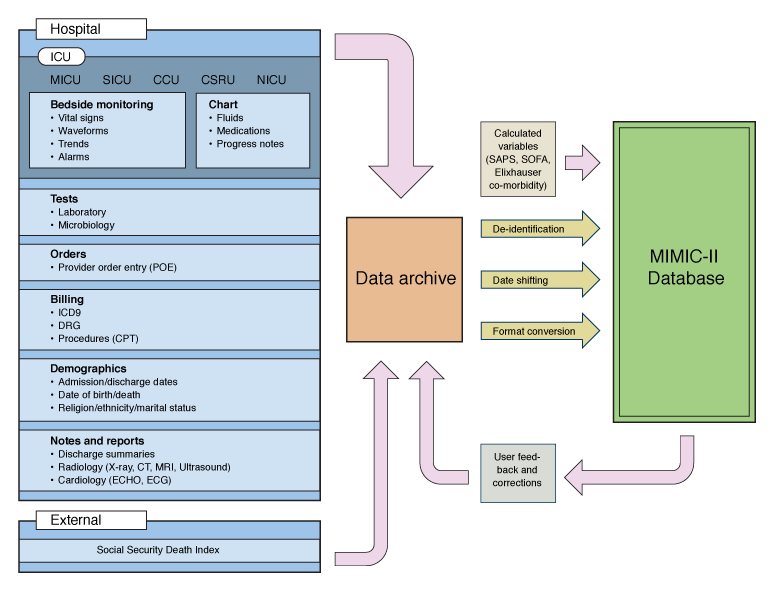
This tutorial explores the Multiparameter Intelligent Monitoring in Intensive Care II (MIMIC-II) Indwelling Arterial Catheters (IAC) dataset, as subset derived from MIMIC-II, the publicly-accessible critical care database. The database was created for the purpose of a case study in the book “Secondary Analysis of Electronic Health Records”, published by Springer in 2016. In particular, the MIMIC-II IAC dataset was used throughout Chapter 16 (Data Analysis) by Raffa J. et al. to investigate the effectiveness of indwelling arterial catheters in hemodynamically stable patients with respiratory failure for mortality outcomes.
More details on the dataset such as all included features and their description can be found here.
import warnings

warnings.filterwarnings("ignore")
from IPython.display import Image

Image(filename="images/MIMIC-II-database-structure.png", width=400)
In this tutorial we want to explore the MIMIC-II IAC dataset using ehrapy to identify patient groups and their associated features.
The major steps of an analysis with ehrapy include:
Preprocessing and quality control (QC)
Dimensionality reduction
Batch effect identification
Clustering
Additional downstream analysis
Before we start with the analysis of the MIMIC-II IAC dataset, we set up our environment including the import of packages and preparation of the dataset.
Environment setup#
import warnings

warnings.filterwarnings("ignore")

import ehrapy as ep
import ehrdata as ed
import matplotlib.pyplot as plt
import pandas as pd
import seaborn as sns

 ⓘ
ⓘ
MIMIC-II IAC dataset loading#
ehrdata offers several datasets in EHRData format that can be used out of the box.
In this tutorial we will use the MIMIC-II IAC dataset with unencoded features. ehrapy’s default encoding is a simple one-hot encoding in this case. More details on encoding can be seen in the next step.
edata = ed.dt.mimic_2()
edata
EHRData object with n_obs × n_vars × n_t = 1776 × 46 × 1
    shape of .X: (1776, 46)
The MIMIC-II dataset has 1776 patients with 46 features.
Now that we have our EHRData file ready, we can start the analysis using ehrapy and the first step will be to preprocess the dataset.
Analysis using ehrapy#
Preprocessing#
ed.infer_feature_types(edata, binary_as="numeric")
! Feature was detected as categorical features stored numerically. Adjust using `ed.replace_feature_types` if needed.
 Detected feature types for EHRData object with 1776 obs and 46 vars
╠══ 📅 Date features
╠══ 📐 Numerical features
║   ╠══ abg_count
║   ╠══ afib_flg
║   ╠══ age
║   ╠══ aline_flg
║   ╠══ bmi
║   ╠══ bun_first
║   ╠══ cad_flg
║   ╠══ censor_flg
║   ╠══ chf_flg
║   ╠══ chloride_first
║   ╠══ copd_flg
║   ╠══ creatinine_first
║   ╠══ day_28_flg
║   ╠══ day_icu_intime_num
║   ╠══ gender_num
║   ╠══ hgb_first
║   ╠══ hosp_exp_flg
║   ╠══ hospital_los_day
║   ╠══ hour_icu_intime
║   ╠══ hr_1st
║   ╠══ icu_exp_flg
║   ╠══ icu_los_day
║   ╠══ iv_day_1
║   ╠══ liver_flg
║   ╠══ mal_flg
║   ╠══ map_1st
║   ╠══ mort_day_censored
║   ╠══ pco2_first
║   ╠══ platelet_first
║   ╠══ po2_first
║   ╠══ potassium_first
║   ╠══ renal_flg
║   ╠══ resp_flg
║   ╠══ sapsi_first
║   ╠══ sepsis_flg
║   ╠══ service_num
║   ╠══ sodium_first
║   ╠══ sofa_first
║   ╠══ spo2_1st
║   ╠══ stroke_flg
║   ╠══ tco2_first
║   ╠══ temp_1st
║   ╠══ wbc_first
║   ╚══ weight_first
╚══ 🗂️ Categorical features
    ╠══ day_icu_intime (7 categories)
    ╚══ service_unit (3 categories)
Let’s have a closer look at the categorical detected features:
edata[:, "day_icu_intime"].X
ArrayView([['Friday   '],
           ['Saturday '],
           ['Friday   '],
           ...,
           ['Tuesday  '],
           ['Wednesday'],
           ['Monday   ']], shape=(1776, 1), dtype=object)
edata[:, "service_unit"].X
ArrayView([['SICU'],
           ['MICU'],
           ['MICU'],
           ...,
           ['MICU'],
           ['SICU'],
           ['MICU']], shape=(1776, 1), dtype=object)
Categorical features could either already be stored numerically (e.g., as 0/1 for flags) or as another type such as strings. Such categorical features need an encoding. Here, we identify service_unit and day_icu_intime as categorical features stored non-numerically. We will therefore encode them first with one-hot encoding. This ensures that no ordering is preserved for the respective features. ehrapy also offers other encoding functions.
edata = ep.pp.encode(edata, encodings={"one-hot": ["service_unit", "day_icu_intime"]})
edata
EHRData object with n_obs × n_vars × n_t = 1776 × 54 × 1
    obs: 'service_unit', 'day_icu_intime'
    var: 'feature_type', 'unencoded_var_names', 'encoding_mode'
    layers: 'original'
    shape of .X: (1776, 54)
    shape of .original: (1776, 54)
ed.feature_type_overview(edata)
 Detected feature types for EHRData object with 1776 obs and 54 vars
╠══ 📅 Date features
╠══ 📐 Numerical features
║   ╠══ abg_count
║   ╠══ afib_flg
║   ╠══ age
║   ╠══ aline_flg
║   ╠══ bmi
║   ╠══ bun_first
║   ╠══ cad_flg
║   ╠══ censor_flg
║   ╠══ chf_flg
║   ╠══ chloride_first
║   ╠══ copd_flg
║   ╠══ creatinine_first
║   ╠══ day_28_flg
║   ╠══ day_icu_intime_num
║   ╠══ gender_num
║   ╠══ hgb_first
║   ╠══ hosp_exp_flg
║   ╠══ hospital_los_day
║   ╠══ hour_icu_intime
║   ╠══ hr_1st
║   ╠══ icu_exp_flg
║   ╠══ icu_los_day
║   ╠══ iv_day_1
║   ╠══ liver_flg
║   ╠══ mal_flg
║   ╠══ map_1st
║   ╠══ mort_day_censored
║   ╠══ pco2_first
║   ╠══ platelet_first
║   ╠══ po2_first
║   ╠══ potassium_first
║   ╠══ renal_flg
║   ╠══ resp_flg
║   ╠══ sapsi_first
║   ╠══ sepsis_flg
║   ╠══ service_num
║   ╠══ sodium_first
║   ╠══ sofa_first
║   ╠══ spo2_1st
║   ╠══ stroke_flg
║   ╠══ tco2_first
║   ╠══ temp_1st
║   ╠══ wbc_first
║   ╚══ weight_first
╚══ 🗂️ Categorical features
    ╠══ day_icu_intime (7 categories); one-hot encoded
    ╚══ service_unit (3 categories); one-hot encoded
Quality Control (QC)#
Demographics distribution#
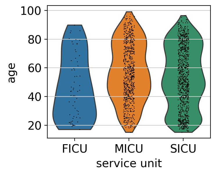
To see if we have strong differences by demographics, we can check these features in a violin plot.
plt.rcParams["figure.figsize"] = (4, 3)
plt.rcParams["figure.dpi"] = 100
ep.pl.violin(edata, keys=["age"], groupby="service_unit")
Missing values#
ehrapy’s pp.qc_metrics() function will calculate several useful metrics such as the absolute number and percentages of missing values and properties like the mean/median/min/max of all features. The percentage of missing values is important as features with too many missing values should not be included.
obs_metric, var_metrics = ep.pp.qc_metrics(edata)
obs_metric
| missing_values_abs | missing_values_pct | entropy_of_missingness | unique_values_abs | unique_values_ratio | |
|---|---|---|---|---|---|
| 0 | 0 | 0.000000 | 3.466198e-09 | 4 | 40.0 |
| 1 | 12 | 22.222222 | 7.642045e-01 | 4 | 40.0 |
| 2 | 0 | 0.000000 | 3.466198e-09 | 4 | 40.0 |
| 3 | 3 | 5.555556 | 3.095434e-01 | 4 | 40.0 |
| 4 | 0 | 0.000000 | 3.466198e-09 | 4 | 40.0 |
| ... | ... | ... | ... | ... | ... |
| 1771 | 1 | 1.851852 | 1.330396e-01 | 4 | 40.0 |
| 1772 | 1 | 1.851852 | 1.330396e-01 | 4 | 40.0 |
| 1773 | 3 | 5.555556 | 3.095434e-01 | 4 | 40.0 |
| 1774 | 1 | 1.851852 | 1.330396e-01 | 4 | 40.0 |
| 1775 | 1 | 1.851852 | 1.330396e-01 | 4 | 40.0 |
1776 rows × 5 columns
var_metrics
| missing_values_abs | missing_values_pct | entropy_of_missingness | unique_values_abs | unique_values_ratio | coefficient_of_variation | is_constant | constant_variable_ratio | range_ratio | mean | median | standard_deviation | min | max | iqr_outliers | |
|---|---|---|---|---|---|---|---|---|---|---|---|---|---|---|---|
| ehrapycat_service_unit_FICU | 0 | 0.000000 | 3.466198e-09 | 3.0 | 0.168919 | NaN | NaN | 2.272727 | NaN | NaN | NaN | NaN | NaN | NaN | True |
| ehrapycat_service_unit_MICU | 0 | 0.000000 | 3.466198e-09 | 3.0 | 0.168919 | NaN | NaN | 2.272727 | NaN | NaN | NaN | NaN | NaN | NaN | True |
| ehrapycat_service_unit_SICU | 0 | 0.000000 | 3.466198e-09 | 3.0 | 0.168919 | NaN | NaN | 2.272727 | NaN | NaN | NaN | NaN | NaN | NaN | True |
| ehrapycat_day_icu_intime_Friday | 0 | 0.000000 | 3.466198e-09 | 7.0 | 0.394144 | NaN | NaN | 2.272727 | NaN | NaN | NaN | NaN | NaN | NaN | True |
| ehrapycat_day_icu_intime_Monday | 0 | 0.000000 | 3.466198e-09 | 7.0 | 0.394144 | NaN | NaN | 2.272727 | NaN | NaN | NaN | NaN | NaN | NaN | True |
| ehrapycat_day_icu_intime_Saturday | 0 | 0.000000 | 3.466198e-09 | 7.0 | 0.394144 | NaN | NaN | 2.272727 | NaN | NaN | NaN | NaN | NaN | NaN | True |
| ehrapycat_day_icu_intime_Sunday | 0 | 0.000000 | 3.466198e-09 | 7.0 | 0.394144 | NaN | NaN | 2.272727 | NaN | NaN | NaN | NaN | NaN | NaN | True |
| ehrapycat_day_icu_intime_Thursday | 0 | 0.000000 | 3.466198e-09 | 7.0 | 0.394144 | NaN | NaN | 2.272727 | NaN | NaN | NaN | NaN | NaN | NaN | True |
| ehrapycat_day_icu_intime_Tuesday | 0 | 0.000000 | 3.466198e-09 | 7.0 | 0.394144 | NaN | NaN | 2.272727 | NaN | NaN | NaN | NaN | NaN | NaN | True |
| ehrapycat_day_icu_intime_Wednesday | 0 | 0.000000 | 3.466198e-09 | 7.0 | 0.394144 | NaN | NaN | 2.272727 | NaN | NaN | NaN | NaN | NaN | NaN | True |
| aline_flg | 0 | 0.000000 | 3.466198e-09 | NaN | NaN | 0.897150 | 0.0 | 2.272727 | 180.487805 | 0.554054 | 1.000000 | 0.497070 | 0.000000 | 1.000000 | False |
| icu_los_day | 0 | 0.000000 | 3.466198e-09 | NaN | NaN | 1.002635 | 0.0 | 2.272727 | 828.926295 | 3.346498 | 2.185000 | 3.355316 | 0.500000 | 28.240000 | True |
| hospital_los_day | 0 | 0.000000 | 3.466198e-09 | NaN | NaN | 1.005417 | 0.0 | 2.272727 | 1368.524818 | 8.110923 | 6.000000 | 8.154862 | 1.000000 | 112.000000 | True |
| age | 0 | 0.000000 | 3.466198e-09 | NaN | NaN | 0.387221 | 0.0 | 2.272727 | 154.342114 | 54.379660 | 53.678585 | 21.056923 | 15.180230 | 99.110947 | False |
| gender_num | 1 | 0.056306 | 6.890036e-03 | NaN | NaN | 0.855399 | 0.0 | 2.272727 | 173.170732 | 0.577465 | 1.000000 | 0.493963 | 0.000000 | 1.000000 | False |
| weight_first | 110 | 6.193694 | 3.350863e-01 | NaN | NaN | 0.280781 | 0.0 | 2.272727 | 284.230173 | 80.075948 | 77.000000 | 22.483765 | 30.000000 | 257.600006 | True |
| bmi | 466 | 26.238739 | 8.303276e-01 | NaN | NaN | 0.294924 | 0.0 | 2.272727 | 309.092904 | 27.827316 | 26.324846 | 8.206940 | 12.784877 | 98.797134 | True |
| sapsi_first | 85 | 4.786036 | 2.772374e-01 | NaN | NaN | 0.290953 | 0.0 | 2.272727 | 205.141184 | 14.136606 | 14.000000 | 4.113085 | 3.000000 | 32.000000 | True |
| sofa_first | 6 | 0.337838 | 3.260037e-02 | NaN | NaN | 0.400970 | 0.0 | 2.272727 | 292.050859 | 5.820904 | 6.000000 | 2.334006 | 0.000000 | 17.000000 | True |
| service_num | 0 | 0.000000 | 3.466198e-09 | NaN | NaN | 0.899196 | 0.0 | 2.272727 | 180.855397 | 0.552928 | 1.000000 | 0.497191 | 0.000000 | 1.000000 | False |
| day_icu_intime_num | 0 | 0.000000 | 3.466198e-09 | NaN | NaN | 0.491831 | 0.0 | 2.272727 | 148.000000 | 4.054054 | 4.000000 | 1.993911 | 1.000000 | 7.000000 | False |
| hour_icu_intime | 0 | 0.000000 | 3.466198e-09 | NaN | NaN | 0.748445 | 0.0 | 2.272727 | 217.276596 | 10.585586 | 9.000000 | 7.922733 | 0.000000 | 23.000000 | False |
| hosp_exp_flg | 0 | 0.000000 | 3.466198e-09 | NaN | NaN | 2.505731 | 0.0 | 2.272727 | 727.868852 | 0.137387 | 0.000000 | 0.344256 | 0.000000 | 1.000000 | True |
| icu_exp_flg | 0 | 0.000000 | 3.466198e-09 | NaN | NaN | 3.073607 | 0.0 | 2.272727 | 1044.705882 | 0.095721 | 0.000000 | 0.294208 | 0.000000 | 1.000000 | True |
| day_28_flg | 0 | 0.000000 | 3.466198e-09 | NaN | NaN | 2.296871 | 0.0 | 2.272727 | 627.561837 | 0.159347 | 0.000000 | 0.365999 | 0.000000 | 1.000000 | True |
| mort_day_censored | 0 | 0.000000 | 3.466198e-09 | NaN | NaN | 0.655993 | 0.0 | 2.272727 | 503.651288 | 614.329825 | 731.000000 | 402.996046 | 0.000000 | 3094.080078 | True |
| censor_flg | 0 | 0.000000 | 3.466198e-09 | NaN | NaN | 1.604195 | 0.0 | 2.272727 | 357.344064 | 0.279842 | 0.000000 | 0.448922 | 0.000000 | 1.000000 | False |
| sepsis_flg | 0 | 0.000000 | 3.466198e-09 | NaN | NaN | NaN | 1.0 | 2.272727 | NaN | 0.000000 | 0.000000 | 0.000000 | 0.000000 | 0.000000 | False |
| chf_flg | 0 | 0.000000 | 3.466198e-09 | NaN | NaN | 2.708880 | 0.0 | 2.272727 | 833.802817 | 0.119932 | 0.000000 | 0.324883 | 0.000000 | 1.000000 | True |
| afib_flg | 0 | 0.000000 | 3.466198e-09 | NaN | NaN | 2.753127 | 0.0 | 2.272727 | 857.971014 | 0.116554 | 0.000000 | 0.320888 | 0.000000 | 1.000000 | True |
| renal_flg | 0 | 0.000000 | 3.466198e-09 | NaN | NaN | 5.347897 | 0.0 | 2.272727 | 2960.000000 | 0.033784 | 0.000000 | 0.180672 | 0.000000 | 1.000000 | True |
| liver_flg | 0 | 0.000000 | 3.466198e-09 | NaN | NaN | 4.115749 | 0.0 | 2.272727 | 1793.939394 | 0.055743 | 0.000000 | 0.229425 | 0.000000 | 1.000000 | True |
| copd_flg | 0 | 0.000000 | 3.466198e-09 | NaN | NaN | 3.211246 | 0.0 | 2.272727 | 1131.210191 | 0.088401 | 0.000000 | 0.283877 | 0.000000 | 1.000000 | True |
| cad_flg | 0 | 0.000000 | 3.466198e-09 | NaN | NaN | 3.665927 | 0.0 | 2.272727 | 1443.902439 | 0.069257 | 0.000000 | 0.253890 | 0.000000 | 1.000000 | True |
| stroke_flg | 0 | 0.000000 | 3.466198e-09 | NaN | NaN | 2.645751 | 0.0 | 2.272727 | 800.000000 | 0.125000 | 0.000000 | 0.330719 | 0.000000 | 1.000000 | True |
| mal_flg | 0 | 0.000000 | 3.466198e-09 | NaN | NaN | 2.436699 | 0.0 | 2.272727 | 693.750000 | 0.144144 | 0.000000 | 0.351236 | 0.000000 | 1.000000 | True |
| resp_flg | 0 | 0.000000 | 3.466198e-09 | NaN | NaN | 1.464023 | 0.0 | 2.272727 | 314.336283 | 0.318131 | 0.000000 | 0.465751 | 0.000000 | 1.000000 | False |
| map_1st | 0 | 0.000000 | 3.466198e-09 | NaN | NaN | 0.199335 | 0.0 | 2.272727 | 215.304774 | 88.246998 | 87.000000 | 17.590711 | 5.000000 | 195.000000 | True |
| hr_1st | 0 | 0.000000 | 3.466198e-09 | NaN | NaN | 0.213315 | 0.0 | 2.272727 | 145.595214 | 87.914977 | 87.000000 | 18.753561 | 30.000000 | 158.000000 | True |
| temp_1st | 3 | 0.168919 | 1.799143e-02 | NaN | NaN | 0.046420 | 0.0 | 2.272727 | 74.443573 | 97.792194 | 98.099998 | 4.539520 | 32.000000 | 104.800003 | True |
| spo2_1st | 0 | 0.000000 | 3.466198e-09 | NaN | NaN | 0.055986 | 0.0 | 2.272727 | 97.528272 | 98.432995 | 100.000000 | 5.510842 | 4.000000 | 100.000000 | True |
| abg_count | 0 | 0.000000 | 3.466198e-09 | NaN | NaN | 1.450669 | 0.0 | 2.272727 | 1921.535422 | 5.984797 | 3.000000 | 8.681962 | 0.000000 | 115.000000 | True |
| wbc_first | 8 | 0.450450 | 4.159395e-02 | NaN | NaN | 0.535533 | 0.0 | 2.272727 | 889.825324 | 12.320396 | 11.300000 | 6.597979 | 0.170000 | 109.800003 | True |
| hgb_first | 8 | 0.450450 | 4.159395e-02 | NaN | NaN | 0.175353 | 0.0 | 2.272727 | 135.441076 | 12.551584 | 12.700000 | 2.200953 | 2.000000 | 19.000000 | True |
| platelet_first | 8 | 0.450450 | 4.159395e-02 | NaN | NaN | 0.405705 | 0.0 | 2.272727 | 398.645751 | 246.083145 | 239.000000 | 99.837223 | 7.000000 | 988.000000 | True |
| sodium_first | 5 | 0.281532 | 2.790864e-02 | NaN | NaN | 0.033856 | 0.0 | 2.272727 | 42.992568 | 139.559006 | 140.000000 | 4.724875 | 105.000000 | 165.000000 | True |
| potassium_first | 5 | 0.281532 | 2.790864e-02 | NaN | NaN | 0.193421 | 0.0 | 2.272727 | 192.325356 | 4.107623 | 4.000000 | 0.794499 | 1.900000 | 9.800000 | True |
| tco2_first | 5 | 0.281532 | 2.790864e-02 | NaN | NaN | 0.204400 | 0.0 | 2.272727 | 245.733883 | 24.416657 | 24.000000 | 4.990763 | 2.000000 | 62.000000 | True |
| chloride_first | 5 | 0.281532 | 2.790864e-02 | NaN | NaN | 0.055207 | 0.0 | 2.272727 | 52.966574 | 103.839074 | 104.000000 | 5.732664 | 78.000000 | 133.000000 | True |
| bun_first | 5 | 0.281532 | 2.790864e-02 | NaN | NaN | 0.745045 | 0.0 | 2.272727 | 710.661668 | 19.277809 | 15.000000 | 14.362833 | 2.000000 | 139.000000 | True |
| creatinine_first | 6 | 0.337838 | 3.260037e-02 | NaN | NaN | 0.988559 | 0.0 | 2.272727 | 1670.155646 | 1.095706 | 0.900000 | 1.083171 | 0.000000 | 18.299999 | True |
| po2_first | 186 | 10.472973 | 4.838116e-01 | NaN | NaN | 0.636217 | 0.0 | 2.272727 | 268.865305 | 227.623270 | 195.000000 | 144.817841 | 22.000000 | 634.000000 | False |
| pco2_first | 186 | 10.472973 | 4.838116e-01 | NaN | NaN | 0.321934 | 0.0 | 2.272727 | 345.511966 | 43.413836 | 41.000000 | 13.976388 | 8.000000 | 158.000000 | True |
| iv_day_1 | 143 | 8.051802 | 4.040018e-01 | NaN | NaN | 1.033093 | 0.0 | 2.272727 | 857.103450 | 1622.907946 | 1081.529175 | 1676.615567 | 0.000000 | 13910.000000 | True |
All properties will be added to the respective layers. Categorical features can be found in the obs layer, while numerical features are in the var layer of the EHRData object. When inspecting both layers, we see that our QC properties were added for each feature if possible.
edata.obs.head(4)
| service_unit | day_icu_intime | missing_values_abs | missing_values_pct | entropy_of_missingness | unique_values_abs | unique_values_ratio | |
|---|---|---|---|---|---|---|---|
| 0 | SICU | Friday | 0 | 0.000000 | 3.466198e-09 | 4 | 40.0 |
| 1 | MICU | Saturday | 12 | 22.222222 | 7.642045e-01 | 4 | 40.0 |
| 2 | MICU | Friday | 0 | 0.000000 | 3.466198e-09 | 4 | 40.0 |
| 3 | SICU | Saturday | 3 | 5.555556 | 3.095434e-01 | 4 | 40.0 |
edata.var.tail(4)
| feature_type | unencoded_var_names | encoding_mode | missing_values_abs | missing_values_pct | entropy_of_missingness | unique_values_abs | unique_values_ratio | coefficient_of_variation | is_constant | constant_variable_ratio | range_ratio | mean | median | standard_deviation | min | max | iqr_outliers | |
|---|---|---|---|---|---|---|---|---|---|---|---|---|---|---|---|---|---|---|
| creatinine_first | numeric | creatinine_first | NaN | 6 | 0.337838 | 0.032600 | NaN | NaN | 0.988559 | 0.0 | 2.272727 | 1670.155646 | 1.095706 | 0.900000 | 1.083171 | 0.0 | 18.299999 | True |
| po2_first | numeric | po2_first | NaN | 186 | 10.472973 | 0.483812 | NaN | NaN | 0.636217 | 0.0 | 2.272727 | 268.865305 | 227.623270 | 195.000000 | 144.817841 | 22.0 | 634.000000 | False |
| pco2_first | numeric | pco2_first | NaN | 186 | 10.472973 | 0.483812 | NaN | NaN | 0.321934 | 0.0 | 2.272727 | 345.511966 | 43.413836 | 41.000000 | 13.976388 | 8.0 | 158.000000 | True |
| iv_day_1 | numeric | iv_day_1 | NaN | 143 | 8.051802 | 0.404002 | NaN | NaN | 1.033093 | 0.0 | 2.272727 | 857.103450 | 1622.907946 | 1081.529175 | 1676.615567 | 0.0 | 13910.000000 | True |
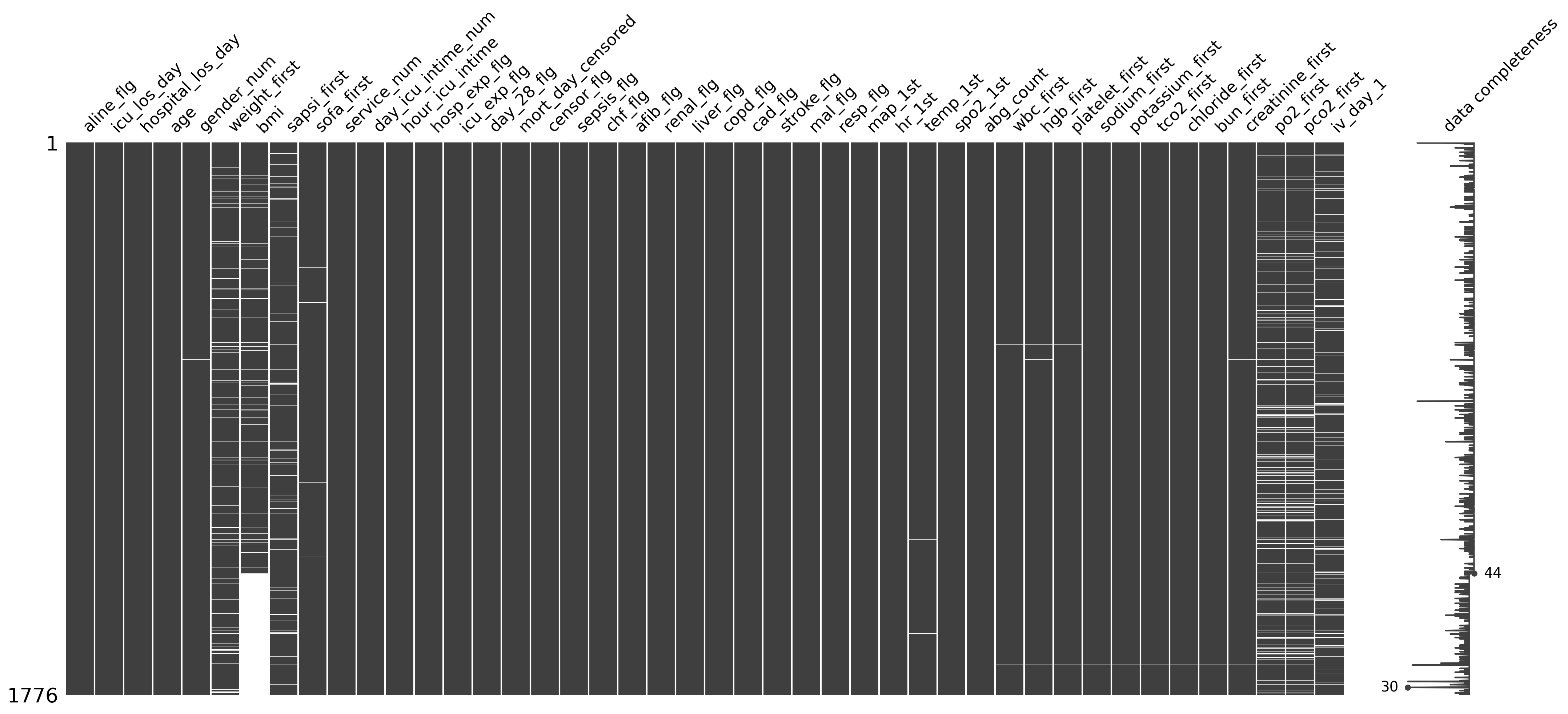
We can visualize the missing values:
ep.pl.missing_values_matrix(edata)
<Axes: >
We can also check which features have the highest percentage of missing values in both obs and vars.
edata.obs.loc[edata.obs["missing_values_pct"] == edata.obs["missing_values_pct"].max(), :]
| service_unit | day_icu_intime | missing_values_abs | missing_values_pct | entropy_of_missingness | unique_values_abs | unique_values_ratio | |
|---|---|---|---|---|---|---|---|
| 1732 | SICU | Thursday | 14 | 25.925926 | 0.825627 | 4 | 40.0 |
| 1751 | MICU | Tuesday | 14 | 25.925926 | 0.825627 | 4 | 40.0 |
edata.var.loc[edata.var["missing_values_pct"] == edata.var["missing_values_pct"].max(), :]
| feature_type | unencoded_var_names | encoding_mode | missing_values_abs | missing_values_pct | entropy_of_missingness | unique_values_abs | unique_values_ratio | coefficient_of_variation | is_constant | constant_variable_ratio | range_ratio | mean | median | standard_deviation | min | max | iqr_outliers | |
|---|---|---|---|---|---|---|---|---|---|---|---|---|---|---|---|---|---|---|
| bmi | numeric | bmi | NaN | 466 | 26.238739 | 0.830328 | NaN | NaN | 0.294924 | 0.0 | 2.272727 | 309.092904 | 27.827316 | 26.324846 | 8.20694 | 12.784877 | 98.797134 | True |
Overall, the percentage of missing values in all features is rather low, however, still some features are not complete.
Features with missing values can introduce a bias in the data, making the processing and analysis challenging. To prevent loss of information due to dropping of multiple features, we can fill up the missing values by performing an imputation. Here, we infer the missing values based on the exisitng part of the data.
To perform this efficiently, we suggest to drop features if the percentage of missing values is very high (>60%). In our data, there is no need to drop any feature, since none exceeds more than 27% missing values (BMI, vars).
Missing data imputation#
ehrapy offers many options to impute missing values in an EHRData object.
Here, we use KNN imputation with 5 neighbors (n_neighbors=5, the default value). The KNN algorithm uses proximity to predict the missing values of a feature by finding the k closest neighbors to the missing value and then imputing the missing value based on the non-missing values in the neighborhood.
ehrapy offers two backends for the nearest neighbors search; scikit-learn and faiss. While faiss is faster for large datasets, scikit-learn is robustly reproducible across different machines.
We are interested to impute only numeric variables here. The main reason for this is that for categorical variables, a very natural way of handling missingness instead of is a dedicated category for missing variables.
ep.pp.knn_impute(
    edata, backend="scikit-learn", n_neighbours=5, var_names=edata.var_names[edata.var["feature_type"] == "numeric"]
)
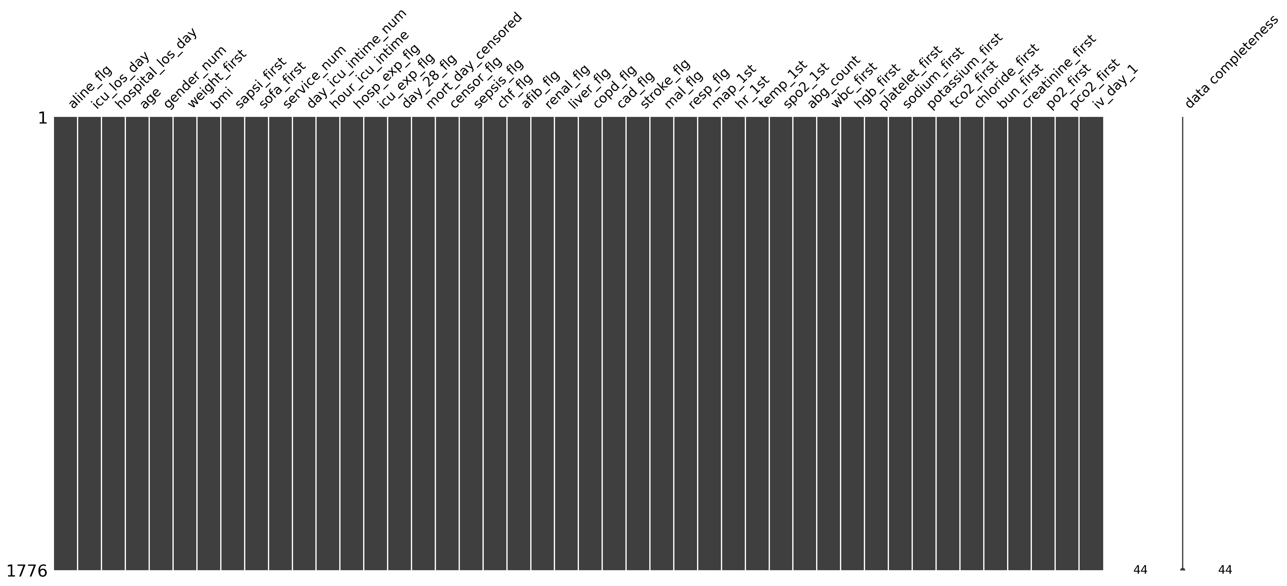
After recalcuating the QC metrices, we can check again the percentage of missing values.
ep.pp.qc_metrics(edata)
ep.pl.missing_values_matrix(edata)
<Axes: >
Data distribution#
Depending on the measurement and the unit of a measurement the value ranges of features may be huge. Clusterings and differential comparisons especially may be greatly influenced by exceptionally big values.
axd = plt.figure(constrained_layout=True, figsize=(8, 3), dpi=100).subplot_mosaic(
    """
    AB
    """
)

sns.histplot(edata.var["min"], ax=axd["A"], bins=30, color="#54C285").set(title="minimum values")
sns.histplot(edata.var["max"], ax=axd["B"], bins=30, color="#1FA6C9").set(title="maximum values")
[Text(0.5, 1.0, 'maximum values')]
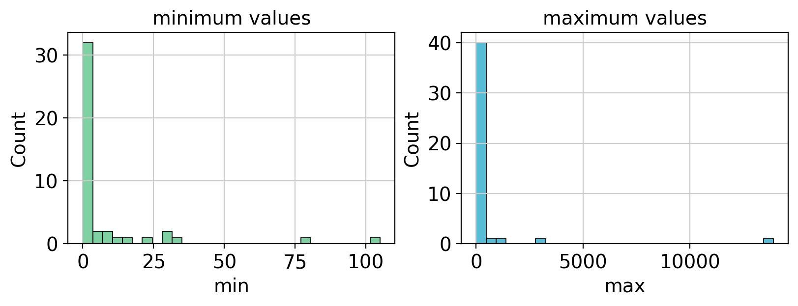
Moreover, features which have a very high coefficient of variation can strongly influence dimensionality reduction. However, since the coefficient of variation performs weak with features that have small means, we only select those which have no small mean.
edata.var["coefficient.variation"] = (edata.var["standard_deviation"] / edata.var["mean"]) * 100
edata.var.loc[(edata.var["coefficient.variation"] > 50) & (edata.var["mean"] > 50),]
| feature_type | unencoded_var_names | encoding_mode | missing_values_abs | missing_values_pct | entropy_of_missingness | unique_values_abs | unique_values_ratio | coefficient_of_variation | is_constant | constant_variable_ratio | range_ratio | mean | median | standard_deviation | min | max | iqr_outliers | coefficient.variation | |
|---|---|---|---|---|---|---|---|---|---|---|---|---|---|---|---|---|---|---|---|
| mort_day_censored | numeric | mort_day_censored | NaN | 0 | 0.0 | 3.466198e-09 | NaN | NaN | 0.655993 | 0.0 | 2.272727 | 503.651288 | 614.329825 | 731.0 | 402.996046 | 0.0 | 3094.080078 | True | 65.599297 |
| po2_first | numeric | po2_first | NaN | 0 | 0.0 | 3.466198e-09 | NaN | NaN | 0.604144 | 0.0 | 2.272727 | 265.742288 | 230.298311 | 204.0 | 139.133431 | 22.0 | 634.000000 | True | 60.414439 |
| iv_day_1 | numeric | iv_day_1 | NaN | 0 | 0.0 | 3.466198e-09 | NaN | NaN | 1.003303 | 0.0 | 2.272727 | 862.094683 | 1613.511866 | 1150.0 | 1618.841925 | 0.0 | 13910.000000 | True | 100.330339 |
The standard deviations and coefficients of variation of the features iv_day_1 (input fluids by IV on day 1 in mL) and po2_first (first PaO_2 in mmHg) are very high with strong spread between minimum and maximum values. These features require normalization.
Normalization#
ehrapy offers several options to normalize data. While it is possible to normalize all numerical values at once with the same normalization function, normalizing only the features with high spread, here iv_day_1 and po2_first, can be sufficient. Log normalization with an offset of 1 to add pseudocounts seems appropriate.
Note: When features with negative values should be normalized you have to use the pp.offset_negative_values() function prior normalization.
ep.pp.log_norm(edata, vars=["iv_day_1", "po2_first"], offset=1)
after normalization we can calculate the QC metrices again and check the distribution.
ep.pp.qc_metrics(edata)
edata.var["coefficient.variation"] = (edata.var["standard_deviation"] / edata.var["mean"]) * 100
edata.var.loc[(edata.var["coefficient.variation"] > 50) & (edata.var["mean"] > 50),]
| feature_type | unencoded_var_names | encoding_mode | missing_values_abs | missing_values_pct | entropy_of_missingness | unique_values_abs | unique_values_ratio | coefficient_of_variation | is_constant | constant_variable_ratio | range_ratio | mean | median | standard_deviation | min | max | iqr_outliers | coefficient.variation | |
|---|---|---|---|---|---|---|---|---|---|---|---|---|---|---|---|---|---|---|---|
| mort_day_censored | numeric | mort_day_censored | NaN | 0 | 0.0 | 3.466198e-09 | NaN | NaN | 0.655993 | 0.0 | 2.272727 | 503.651288 | 614.329825 | 731.0 | 402.996046 | 0.0 | 3094.080078 | True | 65.599297 |
The strong spread of iv_day_1 and po2_first was succesfully removed. Now that we normalized the influence of these features, we can continue with dimensionality reduction.
Dimensionality reduction reduces the number of features (dimensions) by projecting the data to a lower dimensional latent space retaining as much information as possible. This is very useful for high dimensional data, since it reduces complexity and facilitates visualization.
Dimensionality reduction#
Principle Component Analysis (PCA)#
As a next step, we reduce the dimensionality of the dataset with principal component analysis (PCA).
We can also visualize the principal components with ehrapy using the components argument.
scanpy, which ehrapy uses under the hood, provides many options for computing a PCA. The option randomized with a random state is particularly reproducible across different machines. However, different BLAS/LAPACK backends used on different machines have slight differences in SVD. For exact reproducibility, working on in a containerized environment is essential.
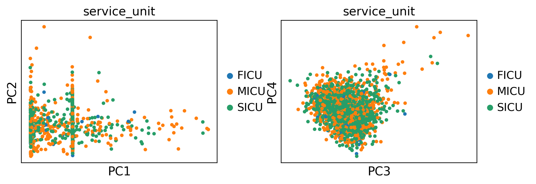
ep.pp.pca(edata, svd_solver="randomized", random_state=42)
ep.pl.pca(edata, color="service_unit", components=["1,2", "3,4"])
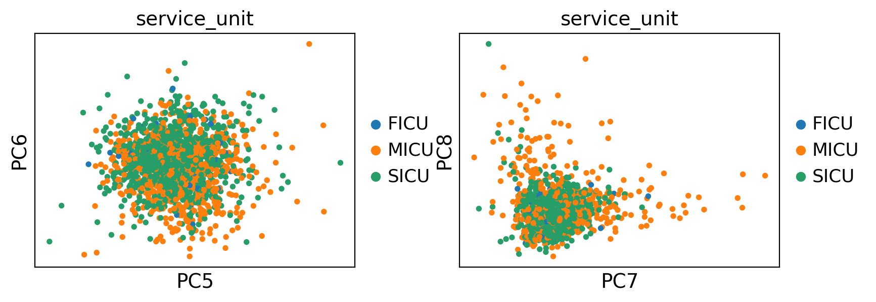
ep.pl.pca(edata, color="service_unit", components=["5,6", "7,8"])
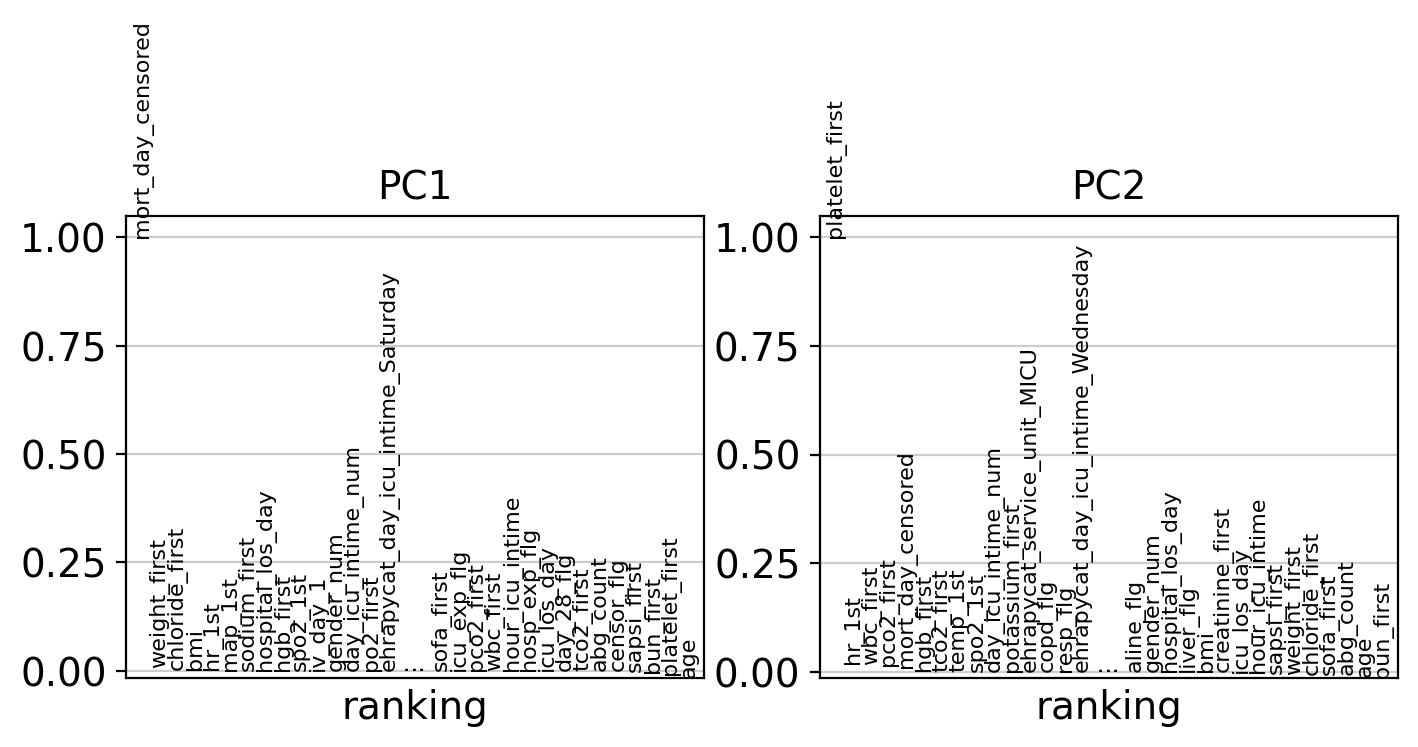
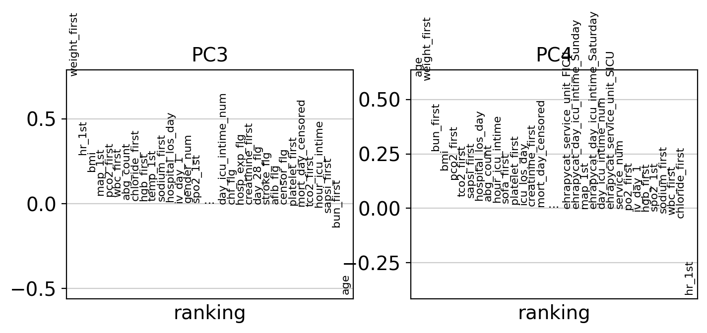
To inspect certain PCs further, we can inspect the PC dimensionality loadings which highlight the features that contribute strongest to the selected PC.
ep.pl.pca_loadings(edata, components="1, 2")
ep.pl.pca_loadings(edata, components="3, 4")
Uniform Manifold Approximation and Projection (UMAP)#
The reduced representation can then be used as input for the neighbors graph calculation which serves as the input for advanced embeddings and visualizations like Uniform Manifold Approximation and Projection (UMAP)
ehrapy provides multiple implementations for neighborhood search. By setting transformer="sklearn", brute-force, but robustly reproducible implementation across machines is available. Faster options for the transformers argument are available, too.
ep.pp.neighbors(edata, transformer="sklearn", n_pcs=10)
ep.tl.umap(edata)
Checking for Batch effects#
Before exploring the data further, we need to see if we have a batch effect. A batch effect can e.g. arise from different collection units or collection days. To check if our data contains a batch for those feautures, we visualize the service_unit and the day_icu_intime.
plt.rcParams["figure.figsize"] = (6, 5)
ep.pl.umap(
    edata,
    color=[
        "service_unit",
        "day_icu_intime",
    ],
    wspace=0.5,
    size=20,
    title=["Service unit", "Day of ICU admission"],
)
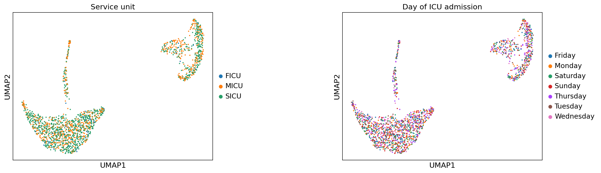
The embeddings suggest that there’s no strong effect by the aforementioned potential confounders.
Selected features on UMAP#
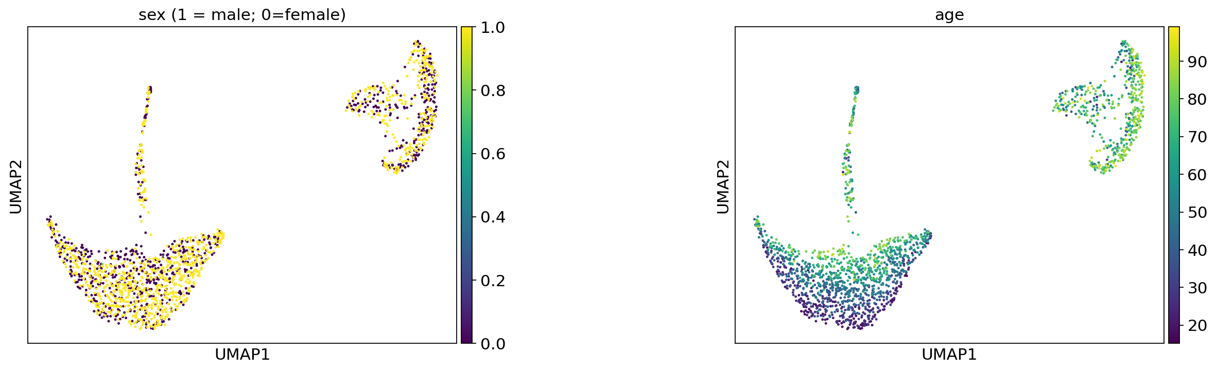
Now we can also highlight other relevant features on the UMAP. Interesting features could be demographics, hospital statistics and lab parameters.
Demographics#
ep.pl.umap(
    edata,
    color=["gender_num", "age"],
    wspace=0.5,
    size=20,
    title=["sex (1 = male; 0=female)", "age"],
)
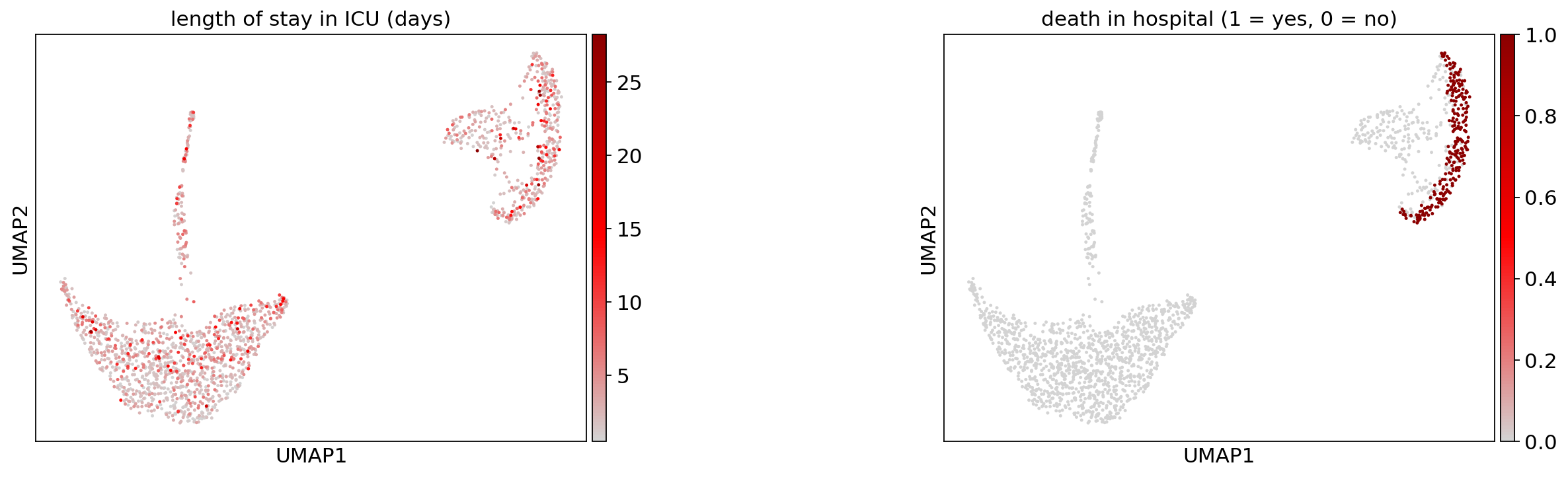
Hospital statistics#
ep.pl.umap(
    edata,
    color=["icu_los_day", "hosp_exp_flg"],
    wspace=0.5,
    size=20,
    cmap=ep.pl.Colormaps.grey_red.value,
    title=["length of stay in ICU (days)", "death in hospital (1 = yes, 0 = no)"],
)
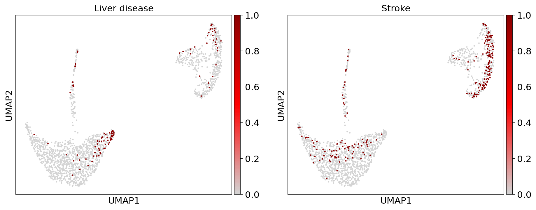
Comorbidities#
ep.pl.umap(
    edata,
    color=["liver_flg", "stroke_flg"],
    cmap=ep.pl.Colormaps.grey_red.value,
    title=["Liver disease", "Stroke"],
    ncols=2,
    size=20,
)
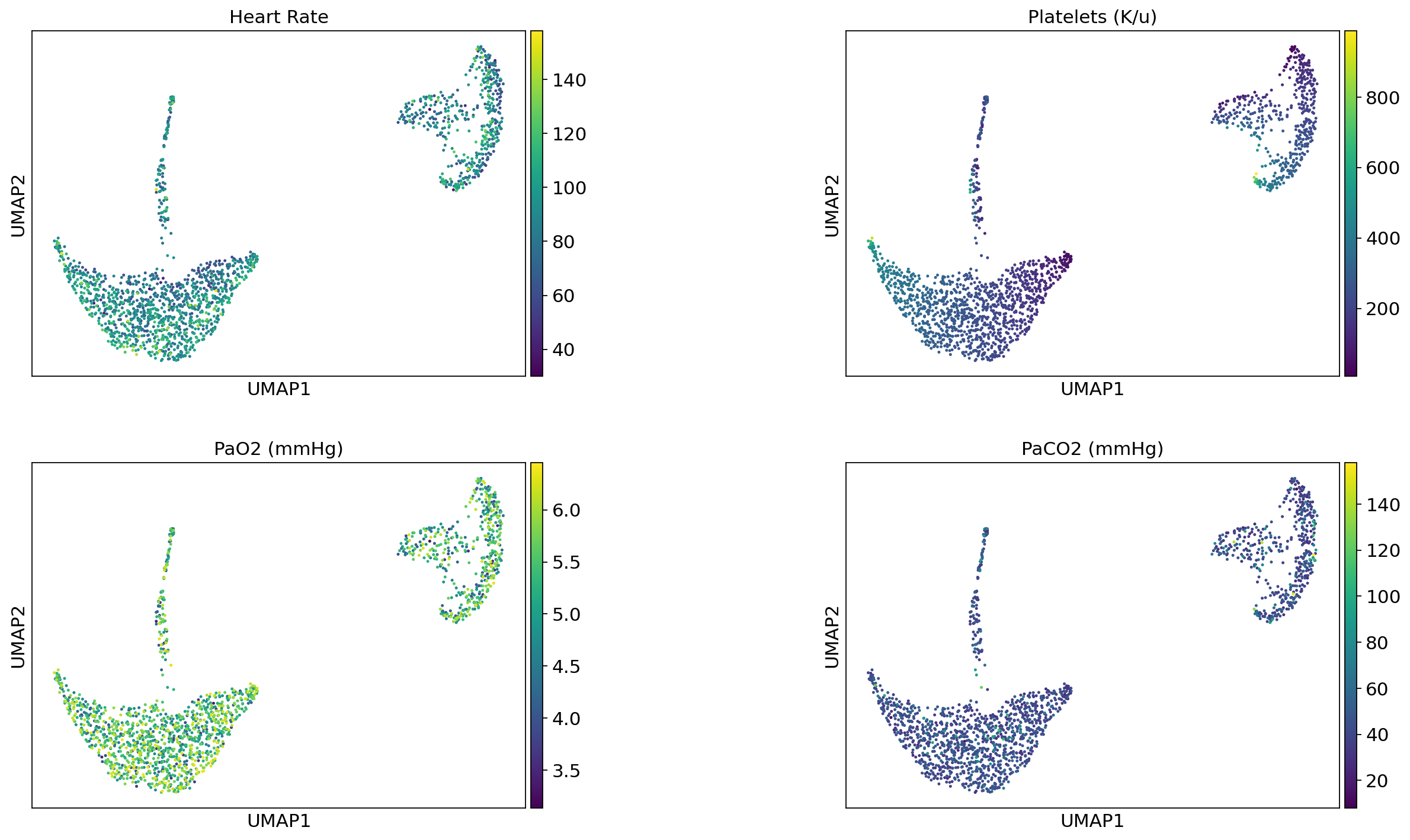
Lab parameters#
ep.pl.umap(
    edata,
    color=["hr_1st", "platelet_first", "po2_first", "pco2_first"],
    wspace=0.5,
    ncols=2,
    size=20,
    title=["Heart Rate", "Platelets (K/u)", "PaO2 (mmHg)", "PaCO2 (mmHg)"],
)
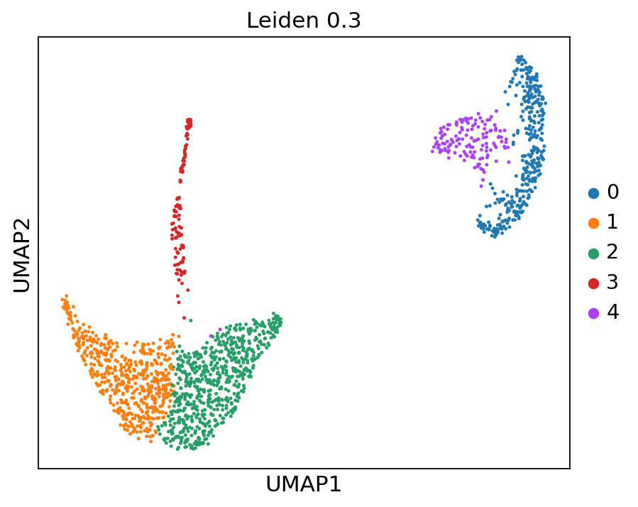
Cluster analysis#
To make more sense of the embedding it is often times useful to determine clusters through e.g. community detection as implemented in the Leiden algorithm. Moreover, clustering allows for unbiased detection of features that are changed between clusters and therefore intersting for us.
Cluster identification#
The implementation in ehrapy allows for the setting of a resolution which determines the number of found clusters. It is often times useful to play around with the parameter.
ep.tl.leiden(edata, resolution=0.3, key_added="leiden_0_3")
The leiden algorithm added a key to obs (leiden_0_3) that stores the clusters. These can subsequently be visualized in the UMAP embedding.
edata.obs.head(4)
| service_unit | day_icu_intime | missing_values_abs | missing_values_pct | entropy_of_missingness | unique_values_abs | unique_values_ratio | leiden_0_3 | |
|---|---|---|---|---|---|---|---|---|
| 0 | SICU | Friday | 0 | 0.0 | 3.466198e-09 | 4 | 40.0 | 0 |
| 1 | MICU | Saturday | 0 | 0.0 | 3.466198e-09 | 4 | 40.0 | 1 |
| 2 | MICU | Friday | 0 | 0.0 | 3.466198e-09 | 4 | 40.0 | 1 |
| 3 | SICU | Saturday | 0 | 0.0 | 3.466198e-09 | 4 | 40.0 | 0 |
ep.pl.umap(edata, color=["leiden_0_3"], title="Leiden 0.3", size=20)
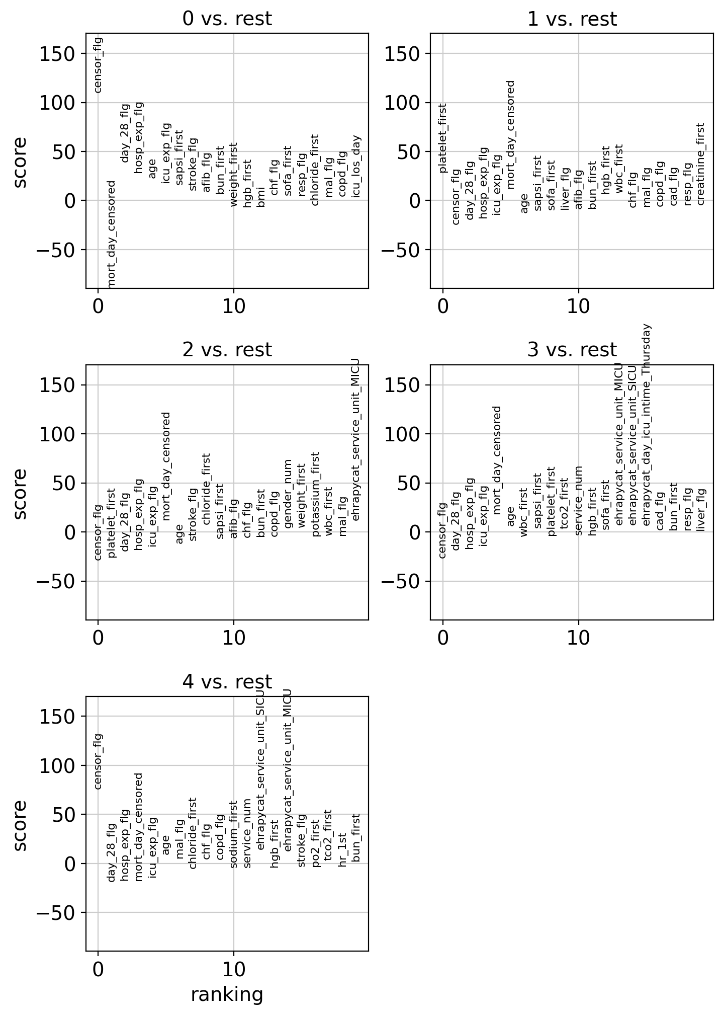
Next, we can explore certain features which are special for certrain clusters and could therefore be used for annotation.
Cluster features#
ep.tl.rank_features_groups(edata, groupby="leiden_0_3")
plt.rcParams["figure.figsize"] = (4, 4)
plt.rcParams["figure.dpi"] = 100
ep.pl.rank_features_groups(edata, key="rank_features_groups", ncols=2)
We can also get the top features per cluster as a DataFrame.
df = ep.get.rank_features_groups_df(edata, group=list(edata.obs["leiden_0_3"].unique()))
df = df.loc[(df["logfoldchanges"] > 0) & (df["pvals_adj"] < 0.05),]
E.g. we can check the top marker of cluster 2.
df.loc[df["group"] == "2",]
| group | names | scores | logfoldchanges | pvals | pvals_adj | |
|---|---|---|---|---|---|---|
| 113 | 2 | mort_day_censored | 12.560957 | inf | 5.805679e-34 | 5.225111e-33 |
| 116 | 2 | chloride_first | 8.095436 | 3.198010 | 1.224180e-15 | 7.345083e-15 |
| 122 | 2 | gender_num | 4.309914 | 0.334411 | 1.747495e-05 | 6.290980e-05 |
| 123 | 2 | weight_first | 4.191347 | 6.553209 | 2.958168e-05 | 9.983817e-05 |
| 127 | 2 | ehrapycat_service_unit_MICU | 11.939801 | 1.000000 | 5.494735e-04 | 1.483579e-03 |
| 129 | 2 | liver_flg | 3.319525 | 1.026702 | 9.328513e-04 | 2.190173e-03 |
| 131 | 2 | iv_day_1 | 3.197073 | 0.415858 | 1.420306e-03 | 3.195689e-03 |
| 132 | 2 | sodium_first | 3.142164 | 1.009302 | 1.709263e-03 | 3.692008e-03 |
| 133 | 2 | service_num | 2.952070 | 0.241071 | 3.210079e-03 | 6.667087e-03 |
| 134 | 2 | ehrapycat_service_unit_SICU | 8.342188 | 1.000000 | 3.873493e-03 | 7.746986e-03 |
| 135 | 2 | bmi | 2.835216 | 1.478226 | 4.650260e-03 | 8.968358e-03 |
| 136 | 2 | sofa_first | 2.582037 | 0.430652 | 9.927681e-03 | 1.848603e-02 |
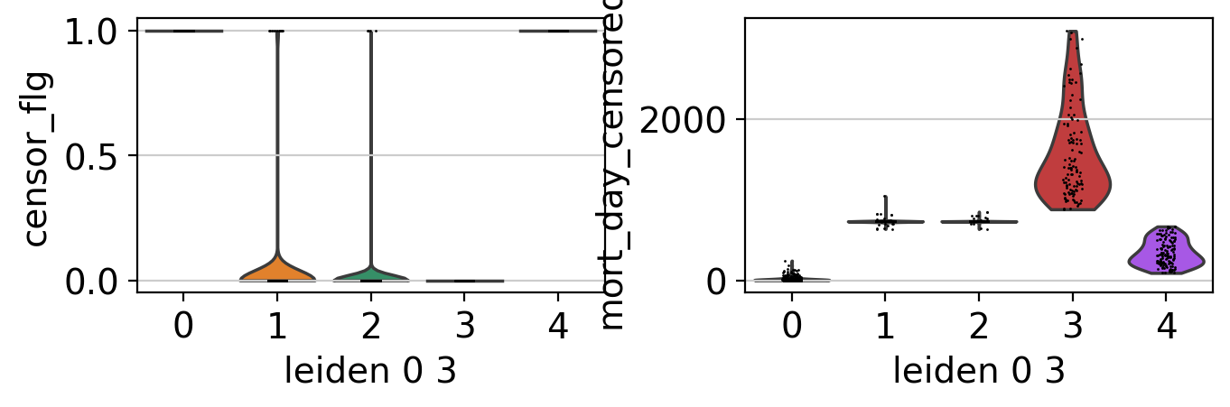
From this table we can also extract the top features in every cluster and highlight those either on the UMAP or as violins plots by cluster.
top_features = df.groupby("group").head(5)
top_features = pd.Series(top_features["names"].unique())
top_features
0                      censor_flg
1                      day_28_flg
2                    hosp_exp_flg
3                             age
4                     icu_exp_flg
5                  platelet_first
6               mort_day_censored
7                       hgb_first
8                       wbc_first
9                          hr_1st
10                 chloride_first
11                     gender_num
12                   weight_first
13    ehrapycat_service_unit_MICU
14                    sapsi_first
15                     tco2_first
16                     sofa_first
17                        mal_flg
18                        chf_flg
19                       copd_flg
dtype: object
plt.rcParams["figure.figsize"] = (3.8, 2)
plt.rcParams["figure.dpi"] = 100
ep.pl.violin(edata, keys=["censor_flg", "mort_day_censored"], groupby="leiden_0_3")
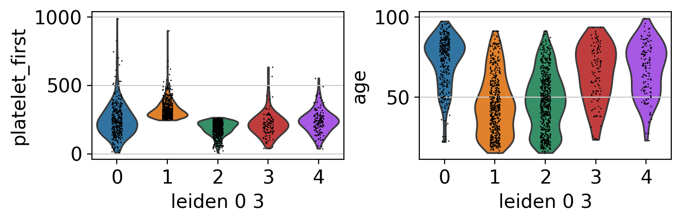
ep.pl.violin(edata, keys=["platelet_first", "age"], groupby="leiden_0_3")
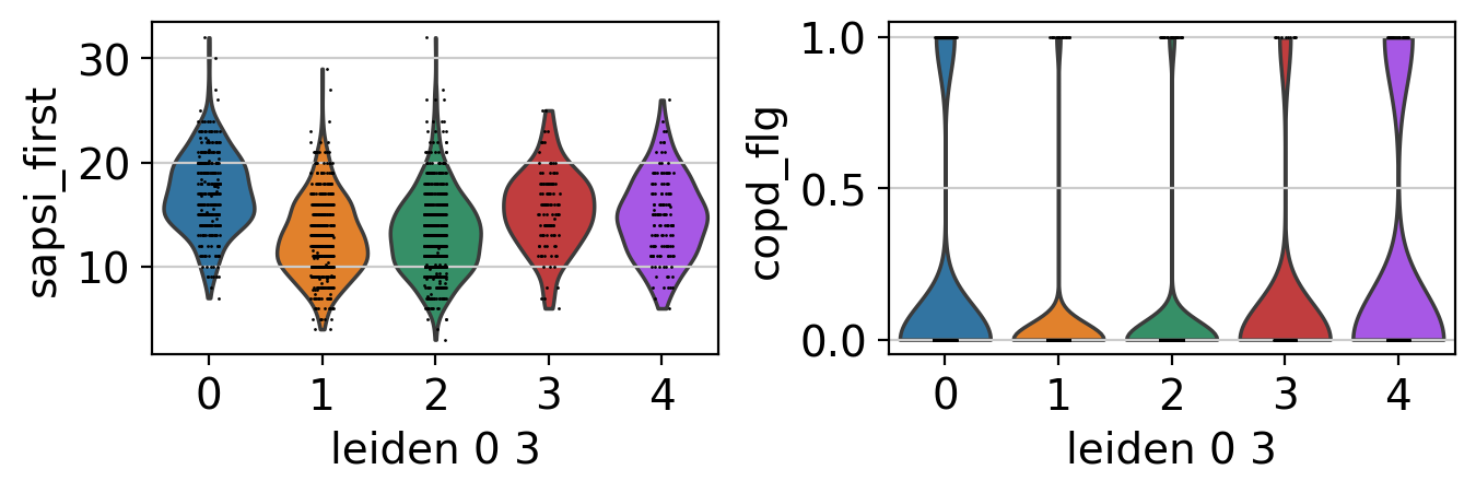
ep.pl.violin(edata, keys=["sapsi_first", "copd_flg"], groupby="leiden_0_3")
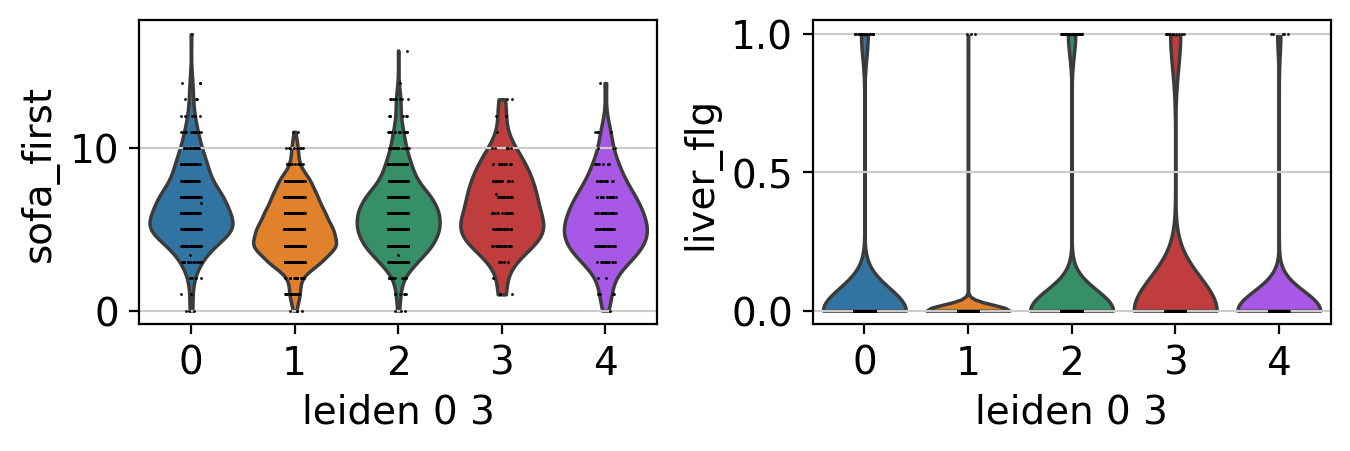
ep.pl.violin(edata, keys=["sofa_first", "liver_flg"], groupby="leiden_0_3")
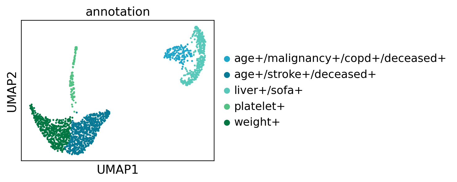
Cluster annotation#
With the knowledge of the cluster features, together with the UMAP plots from above we can annotate the clusters.
edata.obs["annotation"] = "NA"
annotation = {
    "0": "liver+/sofa+",
    "1": "weight+",
    "2": "age+/stroke+/deceased+",
    "3": "platelet+",
    "4": "age+/malignancy+/copd+/deceased+",
    "5": "age+",
}
edata.obs["annotation"] = [annotation[l] if l in annotation.keys() else l for l in edata.obs["leiden_0_3"]]
plt.rcParams["figure.figsize"] = (4, 3)
plt.rcParams["figure.dpi"] = 100
ep.pl.umap(
    edata,
    color="annotation",
    size=20,
    palette={
        "weight+": "#007742",
        "platelet+": "#54C285",
        "age+/stroke+/deceased+": "#087A96",
        "age+/malignancy+/copd+/deceased+": "#1FA6C9",
        "age+": "#F4CC47",
        "liver+/sofa+": "#57C8B9",
        "platelet+/heart_rate+": "#ABEC7D",
    },
)
Additional downstream analysis#
After these basic ehrapy analysis steps, additional downstream analysis can be performed (see also other tutorials).
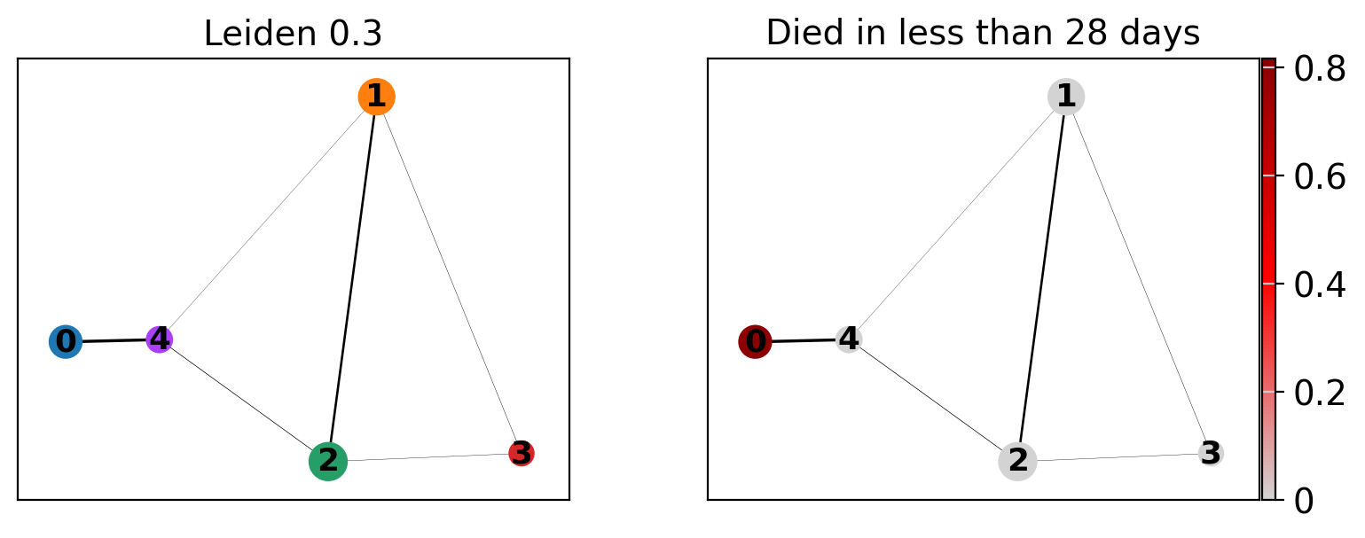
PAGA#
It might also be of interest to infer trajectories to learn about dynamic processes and stage transitions. ehrapy offers several trajectory inference algorithms for this purpose. One of those is partition-based graph abstraction (PAGA).
ep.tl.paga(edata, groups="leiden_0_3")
ep.pl.paga(
    edata,
    color=["leiden_0_3", "day_28_flg"],
    cmap=ep.pl.Colormaps.grey_red.value,
    title=["Leiden 0.3", "Died in less than 28 days"],
)
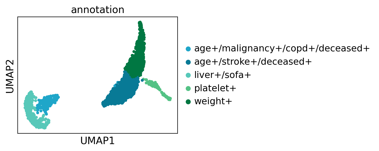
ep.tl.umap(edata, init_pos="paga")
ep.pl.umap(edata, color=["annotation"])
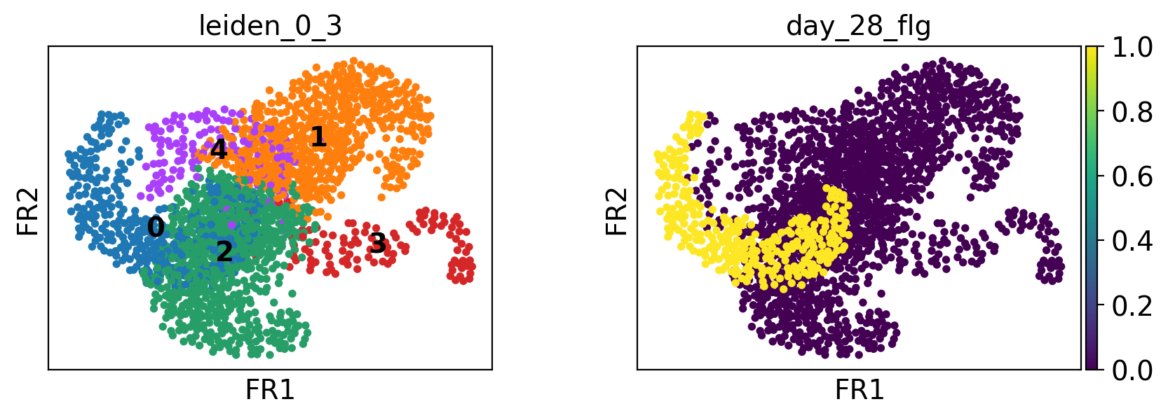
ep.tl.draw_graph(edata, init_pos="paga")
WARNING: Package 'fa2-modified' is not installed, falling back to layout 'fr'.To use the faster and better ForceAtlas2 layout, install package 'fa2-modified' (`pip install fa2-modified`).
ep.tl.draw_graph(edata, init_pos="paga")
ep.pl.draw_graph(edata, color=["leiden_0_3", "day_28_flg"], legend_loc="on data")
WARNING: Package 'fa2-modified' is not installed, falling back to layout 'fr'.To use the faster and better ForceAtlas2 layout, install package 'fa2-modified' (`pip install fa2-modified`).
Exporting results#
We save all of our computations and our final state into an .h5ed file.
It can then be read again using ed.io.read_h5ed.
ed.io.write_h5ed(edata, "mimic_2.h5ed")
Conclusion#
The MIMIC-II IAC dataset comprises electronic health records (EHR) summarized in 46 features from 1776 individuals. This high dimensional data is not easy to interpret and many interesting and previously unknown features can be overseen when just focusing on selected well-defined features. To overcome this hurdle, we applied ehrapy on the MIMIC-II IAC dataset.
ehrapy is based on the EHRData data structure and scanpy pipeline to allow for efficient analysis. We used the build-in functions to preprocess the data, perform QC with imputation of missing data and reduce the dimensionality, resulting in PCA and UMAP embeddings. After performing all these steps, we explored the data by visualizing multiple features on the UMAP embedding, giving a first glance at the patient structure. To identify patient groups in and unbiased fashion, we clustered our data using the Leiden algorithm resulting in 7 different patient clusters. Calculation of cluster-specific features allowed us to annotate the clusters according to the most prominent markers. We saw a strong difference between patients that deceased, had higher age and severe comorbidities such as a stroke and COPD (clusters 2+3) and those that had milder features such as increased platelets and weight (clusters 0+1). Close to these two clusters were two additional clusters that harbored more severe features such as increased heart rate (cluster 5) and high SOFA score with liver disease (cluster 6), indicating potential patient trajectories. Cluster 4 clustered apart from all the others and consists of patients that deceased several months/years after leaving the ICU.
To explore the patient fate, survival and a case study in more detail, continue with our other tutorials or go back to our tutorial overview page.
References#
Raffa, J. (2016). Clinical data from the MIMIC-II database for a case study on indwelling arterial catheters (version 1.0). PhysioNet. https://doi.org/10.13026/C2NC7F.
Raffa J.D., Ghassemi M., Naumann T., Feng M., Hsu D. (2016) Data Analysis. In: Secondary Analysis of Electronic Health Records. Springer, Cham
Goldberger, A., Amaral, L., Glass, L., Hausdorff, J., Ivanov, P. C., Mark, R., … & Stanley, H. E. (2000). PhysioBank, PhysioToolkit, and PhysioNet: Components of a new research resource for complex physiologic signals. Circulation [Online]. 101 (23), pp. e215–e220.
McInnes et al., (2018). UMAP: Uniform Manifold Approximation and Projection. Journal of Open Source Software, 3(29), 861, https://doi.org/10.21105/joss.00861
Traag, V.A., Waltman, L. & van Eck, N.J. From Louvain to Leiden: guaranteeing well-connected communities. Sci Rep 9, 5233 (2019). https://doi.org/10.1038/s41598-019-41695-z
Wolf, F.A., Hamey, F.K., Plass, M. et al. PAGA: graph abstraction reconciles clustering with trajectory inference through a topology preserving map of single cells. Genome Biol 20, 59 (2019). https://doi.org/10.1186/s13059-019-1663-x
Package versions#
!pip list
Package Version Build Editable project location
------------------------- ------------ ----- -----------------------------------------------------------------
aiobotocore 3.2.1
aiofiles 25.1.0
aiohappyeyeballs 2.6.1
aiohttp 3.13.3
aioitertools 0.13.0
aiosignal 1.4.0
anndata 0.12.10
anyio 4.12.1
anywidget 0.9.21
appdirs 1.4.4
argon2-cffi 25.1.0
argon2-cffi-bindings 25.1.0
array-api-compat 1.14.0
arrow 1.4.0
asgiref 3.11.1
asttokens 3.0.1
async-lru 2.2.0
attrs 25.4.0
autograd 1.8.0
autograd-gamma 0.5.0
babel 2.18.0
beautifulsoup4 4.14.3
black 26.3.1
bleach 6.3.0
bokeh 3.8.2
botocore 1.42.61
Bottleneck 1.6.0
causal-learn 0.1.4.4
cellrank 2.2.0
certifi 2026.2.25
cffi 2.0.0
charset-normalizer 3.4.6
clarabel 0.11.1
click 8.3.1
click-log 0.4.0
cloudpickle 3.1.2
colorama 0.4.6
colorcet 3.1.0
comm 0.2.3
contourpy 1.3.3
coverage 7.13.4
cryptography 46.0.5
cuda-bindings 12.9.4
cuda-pathfinder 1.4.2
cvxpy 1.8.1
cycler 0.12.1
Cython 3.2.4
dask 2026.1.2
dask-glm 0.4.0
dask-ml 2025.1.0
debugpy 1.8.20
decorator 5.2.1
defusedxml 0.7.1
deprecation 2.1.0
distributed 2026.1.2
dj-database-url 2.3.0
Django 4.2.29
docrep 0.3.2
docutils 0.22.4
donfig 0.8.1.post1
dotty-dict 1.3.1
dowhy 0.14
dtaidistance 2.4.0
duckdb 1.5.0
ehrapy 0.13.1 /ictstr01/groups/ml01/code/eljas.roellin/ehrapy_workspace/ehrapy
ehrdata 0.1.1 /ictstr01/groups/ml01/code/eljas.roellin/ehrapy_workspace/ehrdata
erdiagram 0.1.3
esbuild_py 0.1.6
et_xmlfile 2.0.0
executing 2.2.1
faiss-cpu 1.13.2
fast-array-utils 1.3.1
fastjsonschema 2.21.2
fhiry 5.2.2
filelock 3.25.2
fknni 1.3.0
fonttools 4.62.1
formulaic 1.2.1
fqdn 1.5.1
frozenlist 1.8.0
fsspec 2026.2.0
generate-tiff-offsets 0.1.9
gitdb 4.0.12
GitPython 3.1.46
google-api-core 2.30.0
google-auth 2.49.1
google-cloud-bigquery 3.40.1
google-cloud-core 2.5.0
google-crc32c 1.8.0
google-resumable-media 2.8.0
googleapis-common-protos 1.73.0
gotrue 1.3.1
graphviz 0.21
greenlet 3.3.2
grpcio 1.78.0
grpcio-status 1.78.0
h11 0.16.0
h5py 3.16.0
highspy 1.13.1
holoviews 1.22.1
httpcore 1.0.9
httpx 0.28.1
icd10-cm 0.0.5
idna 3.11
igraph 1.0.0
ImageIO 2.37.3
importlib_metadata 8.7.1
iniconfig 2.3.0
interface-meta 1.3.0
invoke 1.7.3
ipykernel 7.2.0
ipython 9.11.0
ipython_pygments_lexers 1.1.1
ipywidgets 8.1.8
isoduration 20.11.0
jaraco.classes 3.4.0
jaraco.context 6.1.1
jaraco.functools 4.4.0
jedi 0.19.2
jeepney 0.9.0
Jinja2 3.0.3
jmespath 1.1.0
joblib 1.5.3
json5 0.13.0
jsonpointer 3.0.0
jsonschema 4.26.0
jsonschema-specifications 2025.9.1
jupyter_client 8.8.0
jupyter_core 5.9.1
jupyter-events 0.12.0
jupyter-lsp 2.3.0
jupyter_server 2.17.0
jupyter_server_proxy 4.4.0
jupyter_server_terminals 0.5.4
jupyterlab 4.5.6
jupyterlab_pygments 0.3.0
jupyterlab_server 2.28.0
jupyterlab_widgets 3.0.16
kerchunk 0.2.9
keyring 25.7.0
kiwisolver 1.5.0
lamin_utils 0.9.6
lamindb 0.50.3
lamindb_setup 0.49.7
lark 1.3.1
lazy-loader 0.5
legacy-api-wrap 1.5
leidenalg 0.11.0
lifelines 0.30.3
lightgbm 4.6.0
linkify-it-py 2.1.0
llvmlite 0.46.0
lnschema_core 0.45.2
locket 1.0.0
loompy 3.0.8
Markdown 3.10.2
markdown-it-py 4.0.0
MarkupSafe 3.0.3
matplotlib 3.10.8
matplotlib-inline 0.2.1
mdit-py-plugins 0.5.0
mdurl 0.1.2
miceforest 6.0.5
missingno 0.5.2
mistune 3.2.0
momentchi2 0.1.8
more-itertools 10.8.0
mpmath 1.3.0
msgpack 1.1.2
multidict 6.7.1
multipledispatch 1.0.0
mypy_extensions 1.1.0
narwhals 2.18.0
natsort 8.4.0
nbclient 0.10.4
nbconvert 7.17.0
nbformat 5.10.4
negspy 0.2.24
nest-asyncio 1.6.0
networkx 3.6.1
nh3 0.3.3
notebook_shim 0.2.4
numba 0.64.0
numcodecs 0.16.5
numpy 2.4.3
numpy-groupies 0.11.3
nvidia-cublas-cu12 12.8.4.1
nvidia-cuda-cupti-cu12 12.8.90
nvidia-cuda-nvrtc-cu12 12.8.93
nvidia-cuda-runtime-cu12 12.8.90
nvidia-cudnn-cu12 9.10.2.21
nvidia-cufft-cu12 11.3.3.83
nvidia-cufile-cu12 1.13.1.3
nvidia-curand-cu12 10.3.9.90
nvidia-cusolver-cu12 11.7.3.90
nvidia-cusparse-cu12 12.5.8.93
nvidia-cusparselt-cu12 0.7.1
nvidia-nccl-cu12 2.27.5
nvidia-nvjitlink-cu12 12.8.93
nvidia-nvshmem-cu12 3.4.5
nvidia-nvtx-cu12 12.8.90
ome-zarr 0.12.2
openpyxl 3.1.5
osqp 1.1.1
packaging 26.0
pandas 2.3.3
pandocfilters 1.5.1
panel 1.8.9
param 2.3.2
parso 0.8.6
partd 1.4.2
pathspec 1.0.4
patsy 1.0.2
pexpect 4.9.0
pillow 12.1.1
pip 26.0.1
pkginfo 1.12.1.2
platformdirs 4.9.4
plotly 6.6.0
pluggy 1.6.0
postgrest 0.10.6
prodict 0.8.22
progressbar2 4.5.0
prometheus_client 0.24.1
prompt_toolkit 3.0.52
propcache 0.4.1
proto-plus 1.27.1
protobuf 6.33.5
psutil 7.2.2
psygnal 0.15.1
ptyprocess 0.7.0
pure_eval 0.2.3
pyampute 0.0.3
pyarrow 23.0.1
pyasn1 0.6.2
pyasn1_modules 0.4.2
pycparser 3.0
pydantic 1.10.26
pydot 4.0.1
pygam 0.12.0
Pygments 2.19.2
pygpcca 1.0.4
PyJWT 2.12.1
pynndescent 0.6.0
pyparsing 3.3.2
pytest 9.0.2
pytest-cov 7.0.0
pytest-mock 3.15.1
python-dateutil 2.9.0.post0
python-dotenv 1.2.2
python-gitlab 3.15.0
python-json-logger 4.0.0
python-semantic-release 7.33.2
python-utils 3.9.1
pytokens 0.4.1
pytorch-lightning 2.6.0
pytz 2026.1.post1
pyviz_comms 3.0.6
PyYAML 6.0.3
pyzmq 27.1.0
RapidFuzz 3.14.3
readme_renderer 44.0
realtime 1.0.6
referencing 0.37.0
requests 2.32.5
requests-toolbelt 1.0.0
responses 0.26.0
rfc3339-validator 0.1.4
rfc3986 1.5.0
rfc3986-validator 0.1.1
rfc3987-syntax 1.1.0
rich 14.3.3
rpds-py 0.30.0
s3fs 2026.2.0
scanpy 1.12
scikit-image 0.26.0
scikit-learn 1.8.0
scikit-misc 0.5.2
scipy 1.15.3
scs 3.2.11
scvelo 0.3.4
seaborn 0.13.2
SecretStorage 3.5.0
semver 2.13.0
Send2Trash 2.1.0
sentry-sdk 2.49.0
session-info2 0.4
setuptools 82.0.1
simpervisor 1.0.0
six 1.17.0
smmap 5.0.2
sniffio 1.3.1
sortedcontainers 2.4.0
soupsieve 2.8.3
sparse 0.18.0
SQLAlchemy 1.4.54
sqlparse 0.5.5
stack-data 0.6.3
starlette 0.14.0
statsmodels 0.14.6
storage3 0.5.3
StrEnum 0.4.15
supabase 1.0.3
supafunc 0.2.2
sympy 1.14.0
tableone 0.9.6
tabulate 0.10.0
tblib 3.2.2
tensorly 0.9.0
terminado 0.18.1
texttable 1.7.0
thefuzz 0.22.1
threadpoolctl 3.6.0
tifffile 2026.3.3
timeago 1.0.16
tinycss2 1.4.0
tomlkit 0.14.0
toolz 1.1.0
torch 2.10.0 3
torchmetrics 1.8.2
tornado 6.5.5
tqdm 4.67.3
traitlets 5.14.3
triton 3.6.0
tslearn 0.8.1
twine 3.8.0
typing_extensions 4.15.0
tzdata 2025.3
uc-micro-py 2.0.0
ujson 5.12.0
umap-learn 0.5.11
universal-pathlib 0.1.0
uri-template 1.3.0
urllib3 2.6.3
uvicorn 0.41.0
vitessce 3.5.1
wandb 0.23.1
wcwidth 0.6.0
webcolors 25.10.0
webencodings 0.5.1
websocket-client 1.9.0
websockets 12.0
wheel 0.46.3
widgetsnbextension 4.0.15
wrapt 2.1.2
xarray 2026.2.0
xyzservices 2025.11.0
yarl 1.23.0
zarr 3.1.5
zict 3.0.0
zipp 3.23.0