Longitudinal Data Analysis

This tutorial walks through a longitudinal clinical data analysis workflow:

• EHRData for structured longitudinal clinical data handling

• PyPOTS for time series classification on partially-observed clinical time series

• ehrapy for data exploration, preprocessing, and visualization

• PhysioNet 2012 Challenge dataset for in-hospital mortality prediction

Note

If you’re new to ehrapy and ehrdata, we strongly recommend reading Getting started with ehrdata and Introduction to ehrapy.

Environment setup

import os
import warnings

warnings.filterwarnings("ignore")

# PyPOTS requires this for scipy compatibility
os.environ["SCIPY_ARRAY_API"] = "1"

import ehrapy as ep
import ehrdata as ed
import matplotlib.pyplot as plt
import numpy as np
import seaborn as sns
import torch
from pypots.classification import SAITS
from sklearn.metrics import accuracy_score, auc, confusion_matrix, f1_score, precision_recall_curve, roc_auc_score
from sklearn.model_selection import train_test_split

# Set random seeds for reproducibility
torch.manual_seed(42);

Show code cell output

Hide code cell output

ⓘ

████████╗██╗███╗   ███╗███████╗    ███████╗███████╗██████╗ ██╗███████╗███████╗    █████╗ ██╗
╚══██╔══╝██║████╗ ████║██╔════╝    ██╔════╝██╔════╝██╔══██╗██║██╔════╝██╔════╝   ██╔══██╗██║
   ██║   ██║██╔████╔██║█████╗█████╗███████╗█████╗  ██████╔╝██║█████╗  ███████╗   ███████║██║
   ██║   ██║██║╚██╔╝██║██╔══╝╚════╝╚════██║██╔══╝  ██╔══██╗██║██╔══╝  ╚════██║   ██╔══██║██║
   ██║   ██║██║ ╚═╝ ██║███████╗    ███████║███████╗██║  ██║██║███████╗███████║██╗██║  ██║██║
   ╚═╝   ╚═╝╚═╝     ╚═╝╚══════╝    ╚══════╝╚══════╝╚═╝  ╚═╝╚═╝╚══════╝╚══════╝╚═╝╚═╝  ╚═╝╚═╝
ai4ts v0.0.3 - building AI for unified time-series analysis, https://time-series.ai 

Load PhysioNet 2012 Dataset

edata = ed.dt.physionet2012(layer="tem_data")
edata

View of EHRData object with n_obs × n_vars × n_t = 11988 × 37 × 48
    obs: 'set', 'Age', 'Gender', 'Height', 'ICUType', 'SAPS-I', 'SOFA', 'Length_of_stay', 'Survival', 'In-hospital_death'
    var: 'Parameter'
    tem: '0', '1', '2', '3', '4', '5', '6', '7', '8', '9', '10', '11', '12', '13', '14', '15', '16', '17', '18', '19', '20', '21', '22', '23', '24', '25', '26', '27', '28', '29', '30', '31', '32', '33', '34', '35', '36', '37', '38', '39', '40', '41', '42', '43', '44', '45', '46', '47'
    layers: 'tem_data'
    shape of .tem_data: (11988, 37, 48)

Let’s inspect the data:

edata.obs.head()

	set	Age	Gender	Height	ICUType	SAPS-I	SOFA	Length_of_stay	Survival	In-hospital_death
RecordID
132539	set-a	54.0	0.0	-1.0	4.0	6	1	5	-1	0
132540	set-a	76.0	1.0	175.3	2.0	16	8	8	-1	0
132541	set-a	44.0	0.0	-1.0	3.0	21	11	19	-1	0
132543	set-a	68.0	1.0	180.3	3.0	7	1	9	575	0
132545	set-a	88.0	0.0	-1.0	3.0	17	2	4	918	0

And have a look at the features:

ed.infer_feature_types(edata, layer="tem_data")

! Feature  was detected as categorical features stored numerically. Adjust using `ed.replace_feature_types` if needed.

 Detected feature types for EHRData object with 11988 obs and 37 vars
╠══ 📅 Date features
╠══ 📐 Numerical features
║   ╠══ ALP
║   ╠══ ALT
║   ╠══ AST
║   ╠══ Albumin
║   ╠══ BUN
║   ╠══ Bilirubin
║   ╠══ Cholesterol
║   ╠══ Creatinine
║   ╠══ DiasABP
║   ╠══ FiO2
║   ╠══ GCS
║   ╠══ Glucose
║   ╠══ HCO3
║   ╠══ HCT
║   ╠══ HR
║   ╠══ K
║   ╠══ Lactate
║   ╠══ MAP
║   ╠══ MechVent
║   ╠══ Mg
║   ╠══ NIDiasABP
║   ╠══ NIMAP
║   ╠══ NISysABP
║   ╠══ Na
║   ╠══ PaCO2
║   ╠══ PaO2
║   ╠══ Platelets
║   ╠══ RespRate
║   ╠══ SaO2
║   ╠══ SysABP
║   ╠══ Temp
║   ╠══ TroponinI
║   ╠══ TroponinT
║   ╠══ Urine
║   ╠══ WBC
║   ╠══ Weight
║   ╚══ pH
╚══ 🗂️ Categorical features

Exploratory Data Analysis

We use ehrapy’s inspection tools to understand our cohort and data quality.

Quality control metrics with ehrapy

Before diving into cohort tracking and missing value analysis, we compute quality control (QC) metrics using qc_metrics(). This adds missing-value statistics and summary statistics (mean, median, std, etc.) to edata.obs and edata.var, which supports downstream filtering and interpretation. For longitudinal data we use the tem_data layer.

ep.pp.qc_metrics(edata, layer="tem_data")

print("Observation-level QC (first 5 rows):")
display(edata.obs[["missing_values_abs", "missing_values_pct"]].head())

print("\nVariable-level QC (first 40 rows):")
display(edata.var[["missing_values_pct", "mean", "median", "standard_deviation"]].head(40))

Observation-level QC (first 5 rows):

	missing_values_abs	missing_values_pct
RecordID
132539	1516	85.360360
132540	1375	77.421171
132541	1383	77.871622
132543	1418	79.842342
132545	1472	82.882883

Variable-level QC (first 40 rows):

	missing_values_pct	mean	median	standard_deviation
Parameter
ALP	98.362077	120.142281	82.00	175.242311
ALT	98.315155	362.919577	42.00	1133.465814
AST	98.314982	504.997937	62.00	1649.590278
Albumin	98.741797	2.890663	2.90	0.651872
BUN	92.757688	27.171867	20.00	22.600949
Bilirubin	98.298125	2.864883	0.90	5.770600
Cholesterol	99.827258	155.682093	153.00	44.460024
Creatinine	92.724843	1.473213	1.00	1.550207
DiasABP	45.804833	59.547250	58.00	13.073717
FiO2	84.296971	0.541265	0.50	0.188191
GCS	67.940858	11.415181	13.00	3.993081
Glucose	93.174598	140.844965	127.00	65.012700
HCO3	92.911488	23.154983	23.00	4.721876
HCT	90.495183	30.691727	30.20	5.001046
HR	9.786696	86.615487	86.00	17.858740
K	92.411856	4.128653	4.00	0.680830
Lactate	95.883036	2.954756	2.10	2.565953
MAP	46.114170	80.269169	78.00	16.432571
MechVent	84.923813	1.000000	1.00	0.000000
Mg	92.902277	2.023403	2.00	0.516253
NIDiasABP	57.925808	58.354169	57.00	15.206178
NIMAP	58.505728	77.358974	76.00	15.061055
NISysABP	57.888096	119.687100	117.00	22.430955
Na	92.895500	139.105208	139.00	5.213751
PaCO2	88.459988	40.392285	39.00	9.126968
PaO2	88.481016	147.545456	121.00	85.567716
Platelets	92.629609	189.955339	172.00	107.097081
RespRate	75.935832	19.589149	19.00	5.487177
SaO2	95.984526	96.689699	97.00	3.507824
SysABP	45.800836	119.892138	118.00	23.952596
Temp	62.870162	37.079814	37.10	1.425589
TroponinI	99.795803	8.210383	3.30	10.968970
TroponinT	98.914192	1.174704	0.18	2.786282
Urine	30.718392	115.918911	70.00	158.601586
WBC	93.265835	12.934450	11.50	10.473903
Weight	47.147147	83.091312	80.00	25.130950
pH	87.664401	7.312456	7.38	4.939904

We can see at a glance:

• what percentage of measurements are available on an observation (person) level

• what percentage of measurements are available on a variable level

For the persons, we see from the sample of the first 5 individuals that the missing value percentage, or in other words the monitoring intensity, can vary.

For the variables, we obtain summary statistics (mean, standard deviation) and can spot outliers. The dataset records up to 48 hourly measurements per patient.

The basic physiological measurements — DiasABP, HR, MAP, NIDiasABP, NIMAP, NISysABP, SysABP, Urine, and Weight — are most frequently recorded. More specific measurements like WBC and TroponinI are less frequently measured.

Variable Correlations

After inspecting individual variable quality, we can examine pairwise correlations between variables. This helps identify redundant features, clinically expected relationships, and potential confounders before any preprocessing is applied. Note that correlation estimates for variables with higher missingness are based on fewer observations.

ep.pl.variable_correlations(
    edata,
    layer="tem_data",
    method="pearson",
    correction_method="fdr_bh",
    agg="mean",
    show_values=False,
    width=800,
    height=800,
)

:HeatMap   [variable1,variable2]   (correlation,label)

Cohort Tracking with CohortTracker

Let us examine the information of the cohort in more detail. ehrapy’s CohortTracker records how the cohort changes through each processing step, allowing us to visualize the full pipeline at the end.

tracking_cols = ["Age", "Gender", "ICUType", "SAPS-I", "SOFA", "Length_of_stay", "Survival", "In-hospital_death"]
categorical_cols = ["Gender", "ICUType", "In-hospital_death"]

ct = ep.tl.CohortTracker(edata, columns=tracking_cols, categorical=categorical_cols)
ct(edata, label="Initial Cohort", operations_done="Loaded PhysioNet 2012 dataset")
ct.plot_cohort_barplot()

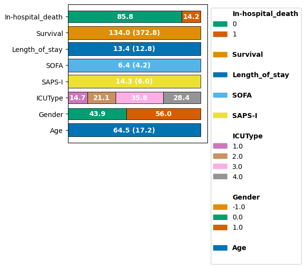
We can observe that on average, patients are 64.5 years old upon ICU entry, with slightly more females (0) than males (1).

Sankey Diagrams for Patient Flow

We can further inspect variables with a Sankey diagram:

ep.pl.sankey_diagram(
    edata,
    columns=["Gender", "In-hospital_death"],
    title="Patient Flow: Gender to Sepsis Status",
)

Where we can obtain a quick visual cue about e.g. the relation of Gender and In-hospital_death.

Here, there is no immediate indication that these two variables are strongly associated in our cohort.

We can also inspect variables longitudinally for how patients change along the time axis. A Sankey diagram is for categorical variables. Since our time-series data consists of continuous variables, we create a quick example with categorized values.

For this, let us explore the heart rate HR, which we bin for a rough overview into low, normal, high, and missing.

# create a new layer in edata
edata.layers["cat_hr"] = edata.layers["tem_data"].copy()

# fill the HR variable (index 14) with the categorical values
edata.layers["cat_hr"][:, 14, :] = np.where(
    edata.layers["tem_data"][:, 14, :] < 60, 0, edata.layers["cat_hr"][:, 14, :]
)
edata.layers["cat_hr"][:, 14, :] = np.where(
    edata.layers["tem_data"][:, 14, :] >= 100, 2, edata.layers["cat_hr"][:, 14, :]
)
edata.layers["cat_hr"][:, 14, :] = np.where(
    (edata.layers["tem_data"][:, 14, :] >= 60) & (edata.layers["tem_data"][:, 14, :] <= 100),
    1,
    edata.layers["cat_hr"][:, 14, :],
)
edata.layers["cat_hr"][:, 14, :] = np.where(
    np.isnan(edata.layers["tem_data"][:, 14, :]), 3, edata.layers["cat_hr"][:, 14, :]
)

Let’s visualize these HR categories for the first 5 hours:

# plot the Sankey diagram
ep.pl.sankey_diagram_time(
    edata[:, :, :5],
    var_name="HR",
    layer="cat_hr",
    state_labels={0: "Low HR", 1: "Normal HR", 2: "High HR", 3: "Missing HR"},
    width=700,
)

{0: 'Low HR', 1: 'Normal HR', 2: 'High HR', 3: 'Missing HR'}
names
['Low HR', 'Normal HR', 'High HR', 'Missing HR']

We can see that most patients at hour 0 (leftmost) have no HR measurement. Further, most patients with measured HR display a normal measurement at hour 0.

We can observe that the fraction of patients with no HR measurement at every hour declines as their ICU stay proceeds.

Time Series Visualization

For exploring continuous variables across time, ehrapy provides timeseries(). Let’s look at a few vital parameters for the first two patients:

vital_vars = ["HR", "SaO2", "Temp", "NISysABP", "NIDiasABP", "RespRate"]

ep.pl.timeseries(
    edata[:2],
    layer="tem_data",
    var_names=vital_vars,
)

We can see that the measurements of vital signs can be very irregular, and different for different individuals. While individual 132540 had their HR constantly monitored, no data on their RespRate is available. Individual 132539 on the other hand has HR and RespRate data available, but multiple gaps where none of these values were acquired.

Normalization

Variables have different scales and units. To focus on within-feature deviation from the population mean rather than on numeric magnitude, we normalize. ehrapy offers multiple normalization approaches; here we use scale_norm() which applies standard (z-score) normalization per feature.

edata.layers["norm_data"] = edata.layers["tem_data"].copy()
ep.pp.scale_norm(edata, layer="norm_data")

vital_vars = ["HR", "SaO2", "Temp", "NISysABP", "NIDiasABP", "RespRate"]
ep.pl.timeseries(
    edata[:2],
    layer="norm_data",
    var_names=vital_vars,
)

Imputation

Clinical time series are often sparsely observed: a patient’s heart rate may be recorded every few minutes, while a lab value like creatinine is only drawn once a day. Last Observation Carried Forward (LOCF) is a simple imputation strategy that fills each missing time point with the most recent observed value, mimicking the clinical assumption that a measurement remains valid until the next reading.

For values missing at the start of the time window (before any observation exists), a fallback_method is used. Here we fall back to the per-feature mean so that no NaNs remain for downstream steps.

ehrapy provides locf_impute() for this directly on 3D EHRData layers:

edata.layers["locf_data"] = edata.layers["norm_data"].copy()
ep.pp.locf_impute(edata, layer="locf_data", fallback_method="mean")

vital_vars = ["HR", "SaO2", "Temp", "NISysABP", "NIDiasABP", "RespRate"]
ep.pl.timeseries(
    edata[:2],
    layer="locf_data",
    var_names=vital_vars,
)

After LOCF imputation the gaps are filled with the last observed reading: plateaus in the time series correspond to periods where a value was carried forward. The initial period (before the first observation) is filled using the population mean as fallback.

Temporal representations

To build a 2D patient-by-feature representation from 3D longitudinal data, we aggregate each variable’s time series into summary statistics (mean and standard deviation across time). This captures both the central tendency and variability of each clinical variable across the full 48-hour stay without relying on an arbitrary single time point.

We use the LOCF-imputed layer from above so that the statistics reflect carried-forward measurements rather than ignoring gaps.

mean_rep = np.nanmean(edata.layers["locf_data"], axis=2)
std_rep = np.nanstd(edata.layers["locf_data"], axis=2)
edata.obsm["temporal_rep"] = np.hstack([mean_rep, std_rep])

ep.pp.neighbors(edata, n_neighbors=15, use_rep="temporal_rep", key_added="temporal_neighbors")
ep.tl.leiden(edata, neighbors_key="temporal_neighbors", key_added="temporal_leiden", resolution=0.2, random_state=0)
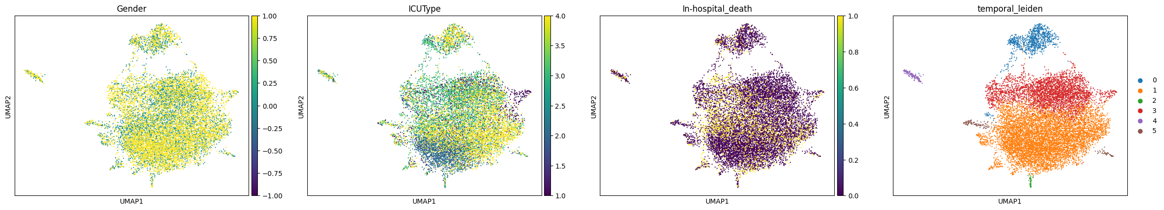
ep.tl.umap(edata, neighbors_key="temporal_neighbors")
ep.pl.umap(edata, color=["Gender", "ICUType", "In-hospital_death", "temporal_leiden"], show=False);

Rank features groups

We identify which static features differ across the Leiden clusters using ep.tl.rank_features_groups. This helps us understand what patient characteristics the unsupervised clustering has captured.

ep.tl.rank_features_groups(
    edata,
    field_to_rank="obs",
    columns_to_rank={"obs_names": ["Age", "Gender", "SAPS-I", "SOFA", "Length_of_stay", "missing_values_pct"]},
    groupby="temporal_leiden",
    key_added="rank_features_groups",
)
ep.pl.rank_features_groups(edata, key="rank_features_groups", n_features=10, show=False);

! Feature  was detected as categorical features stored numerically. Adjust using `ed.replace_feature_types` if needed.
! Detected no columns that need to be encoded. Leaving passed EHRData/AnnData object unchanged.

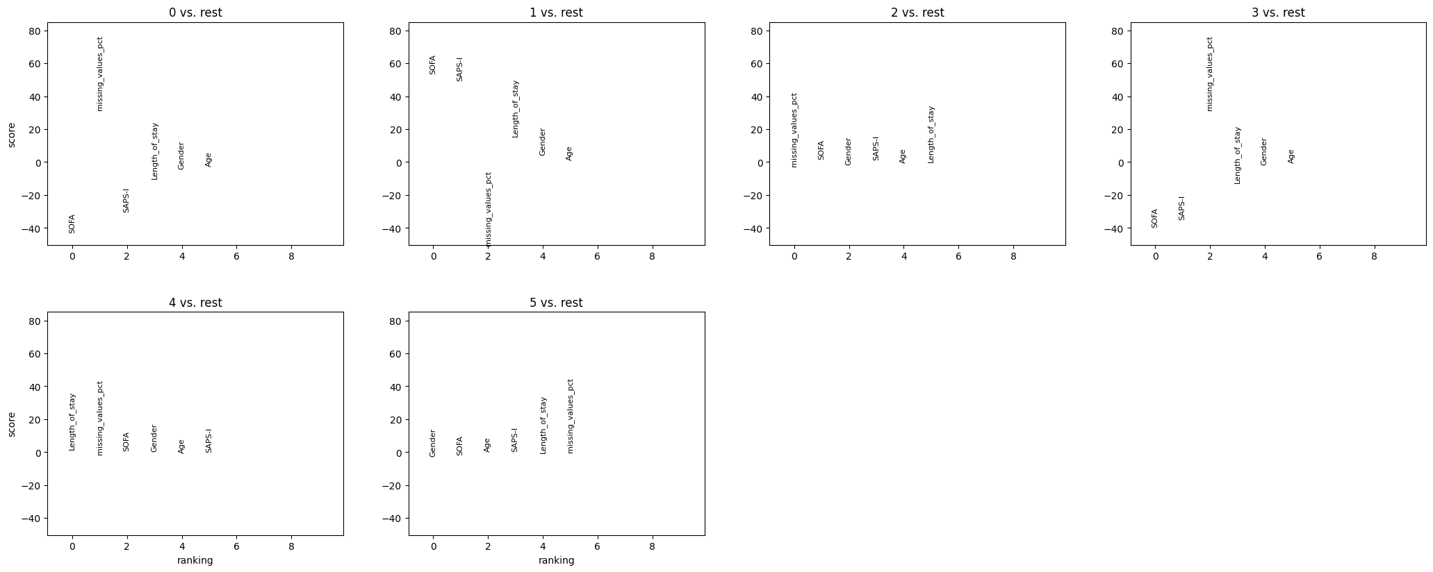
The Leiden clustering, defined entirely on dynamic variables, subgroups patients by severity scores (SOFA, SAPS-I) and monitoring intensity (missing value percentage).

Machine Learning with SAITS

Having explored the data and built unsupervised representations, we now train a deep learning classifier to predict in-hospital mortality.

SAITS (Self-Attention-based Imputation for Time Series) is designed for classification on partially-observed time series, making it well-suited for clinical data where missing values are common. It uses diagonal masked self-attention (DMSA) to jointly handle missingness patterns and temporal dependencies. See the PyPOTS documentation for details.

Data splitting

train_indices = np.arange(len(edata))
train_idx, temp_idx = train_test_split(
    train_indices,
    test_size=0.3,
    random_state=42,
    stratify=edata.obs["SepsisLabel"] if "SepsisLabel" in edata.obs.columns else None,
)
val_idx, test_idx = train_test_split(
    temp_idx,
    test_size=0.5,
    random_state=42,
    stratify=edata.obs.iloc[temp_idx]["SepsisLabel"] if "SepsisLabel" in edata.obs.columns else None,
)

edata_train = edata[train_idx].copy()
edata_val = edata[val_idx].copy()
edata_test = edata[test_idx].copy()

# Track cohort changes
ct(edata_train, label="Training Set", operations_done="Split into train/val/test")

SAITS model configuration

We configure SAITS for the PhysioNet 2012 dataset:

• Sequence length: 48 hourly steps, 37 clinical variables

• Binary classification: in-hospital mortality

• DMSA architecture: 2 layers, d_model=64, n_heads=4

ep.settings.verbosity = "error"

# Initialize SAITS classifier
n_timesteps = edata_train.shape[2]
n_features = edata_train.shape[1]
n_classes = 2  # Binary classification: in-hospital death vs. no in-hospital death

# SAITS architecture: d_model must be divisible by n_heads, d_k = d_model / n_heads
d_model = 64
n_heads = 4
d_k = d_v = d_model // n_heads  # 16

# Initialize SAITS with PyPOTS defaults and reasonable training settings
saits = SAITS(
    n_steps=n_timesteps,
    n_features=n_features,
    n_classes=n_classes,
    # Architecture parameters required by SAITS
    n_layers=2,
    d_model=d_model,
    n_heads=n_heads,
    d_k=d_k,
    d_v=d_v,
    d_ffn=128,
    dropout=0.1,
    attn_dropout=0.1,
    diagonal_attention_mask=True,  # DMSA
    # Training configuration
    epochs=4,
    batch_size=32,
    patience=1,
    device="cuda" if torch.cuda.is_available() else "cpu",
    saving_path="./saits_model",  # Save model checkpoints
)

print(f"\nUsing device: {saits.device}")
print(f"Model initialized with {sum(p.numel() for p in saits.model.parameters())} parameters")

Show code cell output

Hide code cell output

2026-04-10 14:14:35 [INFO]: Using the given device: cpu
2026-04-10 14:14:35 [INFO]: Model files will be saved to ./saits_model/20260410_T141435
2026-04-10 14:14:35 [INFO]: Tensorboard file will be saved to ./saits_model/20260410_T141435/tensorboard
2026-04-10 14:14:35 [INFO]: Using customized CrossEntropy as the training loss function.
2026-04-10 14:14:35 [INFO]: Using customized CrossEntropy as the validation metric function.
2026-04-10 14:14:35 [INFO]: SAITS initialized with the given hyperparameters, the number of trainable parameters: 155,416

Using device: cpu
Model initialized with 155416 parameters

Training

saits.fit(
    train_set={
        "X": edata_train.layers["norm_data"].transpose(0, 2, 1),
        "y": edata_train.obs["In-hospital_death"].values,
    },
    val_set={"X": edata_val.layers["norm_data"].transpose(0, 2, 1), "y": edata_val.obs["In-hospital_death"].values},
)

Show code cell output

Hide code cell output

2026-04-10 14:14:43 [INFO]: Epoch 001 - training loss (CrossEntropy): 0.3636, validation CrossEntropy: 0.2998
2026-04-10 14:14:50 [INFO]: Epoch 002 - training loss (CrossEntropy): 0.3226, validation CrossEntropy: 0.2935
2026-04-10 14:14:57 [INFO]: Epoch 003 - training loss (CrossEntropy): 0.3054, validation CrossEntropy: 0.2897
2026-04-10 14:15:04 [INFO]: Epoch 004 - training loss (CrossEntropy): 0.2963, validation CrossEntropy: 0.3052
2026-04-10 14:15:04 [INFO]: Exceeded the training patience. Terminating the training procedure...
2026-04-10 14:15:04 [INFO]: Finished training. The best model is from epoch#3.
2026-04-10 14:15:04 [INFO]: Saved the model to ./saits_model/20260410_T141435/SAITS.pypots

Model Evaluation

We evaluate the trained model on the held-out test set using standard classification metrics.

# Evaluate the trained SAITS classifier on the test set
test_predictions = saits.predict({"X": edata_test.layers["norm_data"].transpose(0, 2, 1)})

test_pred_labels = test_predictions["classification"]
test_pred_proba = test_predictions["classification_proba"]

y_test = edata_test.obs["In-hospital_death"]
roc_auc = roc_auc_score(y_test, test_pred_proba[:, 1])
precision, recall, _ = precision_recall_curve(y_test, test_pred_proba[:, 1])
pr_auc = auc(recall, precision)
f1 = f1_score(y_test, test_pred_labels)
accuracy = accuracy_score(y_test, test_pred_labels)

print(f"ROC-AUC: {roc_auc:.4f} | PR-AUC: {pr_auc:.4f} | F1: {f1:.4f} | Accuracy: {accuracy:.4f}")

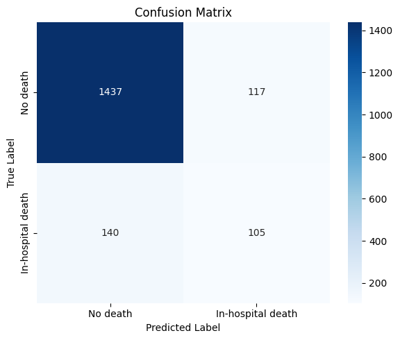
cm = confusion_matrix(y_test, test_pred_labels)
plt.figure(figsize=(6, 5))
sns.heatmap(
    cm,
    annot=True,
    fmt="d",
    cmap="Blues",
    xticklabels=["No death", "In-hospital death"],
    yticklabels=["No death", "In-hospital death"],
)
plt.title("Confusion Matrix")
plt.ylabel("True Label")
plt.xlabel("Predicted Label")
plt.tight_layout()
plt.show()

ROC-AUC: 0.8372 | PR-AUC: 0.4785 | F1: 0.4497 | Accuracy: 0.8571

# Plot ROC and PR curves
fig, (ax1, ax2) = plt.subplots(1, 2, figsize=(14, 5))

# ROC Curve
from sklearn.metrics import roc_curve

fpr, tpr, _ = roc_curve(y_test, test_pred_proba[:, 1])
ax1.plot(fpr, tpr, label=f"SAITS (AUC = {roc_auc:.3f})", linewidth=2)
ax1.plot([0, 1], [0, 1], "k--", label="Random")
ax1.set_xlabel("False Positive Rate", fontsize=12)
ax1.set_ylabel("True Positive Rate", fontsize=12)
ax1.set_title("ROC Curve", fontsize=14)
ax1.legend(fontsize=11)
ax1.grid(alpha=0.3)

# PR Curve
ax2.plot(recall, precision, label=f"SAITS (AUC = {pr_auc:.3f})", linewidth=2)
baseline = y_test.mean()
ax2.plot([0, 1], [baseline, baseline], "k--", label=f"Baseline ({baseline:.3f})")
ax2.set_xlabel("Recall", fontsize=12)
ax2.set_ylabel("Precision", fontsize=12)
ax2.set_title("Precision-Recall Curve", fontsize=14)
ax2.legend(fontsize=11)
ax2.grid(alpha=0.3)

plt.tight_layout()
plt.show()

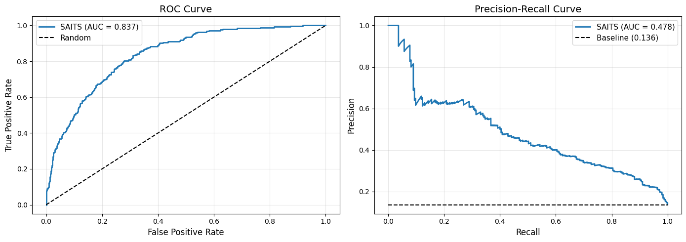
The label imbalance — far more survivors than non-survivors — biases the model towards predicting “no in-hospital death”. The PR curve gives a more informative view of performance on the minority class than the ROC curve.

Exploring SAITS representations

Beyond classification, we can extract the internal representations that SAITS learns. These embeddings encode temporal patterns learned in a supervised fashion, in contrast to the simple statistical aggregation from before. We store them in .obsm and apply the same neighborhood / Leiden / UMAP workflow.

data = edata_test.layers["tem_data"].transpose(0, 2, 1).copy()
missing_mask = np.isnan(data)
data[missing_mask] = 0
data = torch.tensor(data, dtype=torch.float32)

_, _, X_tilde_3, _, _, _ = saits.model.encoder(
    torch.tensor(data, dtype=torch.float32),
    torch.tensor(missing_mask, dtype=torch.float32),
    None,
)

edata_test.obsm["saits_embedding"] = X_tilde_3.mean(dim=1).detach().numpy()

ep.pp.neighbors(edata_test, use_rep="saits_embedding", key_added="saits_neighbors", n_neighbors=15)
ep.tl.leiden(edata_test, neighbors_key="saits_neighbors", key_added="saits_leiden", resolution=0.2, random_state=0)
ep.tl.umap(edata_test, neighbors_key="saits_neighbors")

ep.pl.umap(
    edata_test,
    color=["In-hospital_death", "temporal_leiden", "saits_leiden"],
    show=False,
);

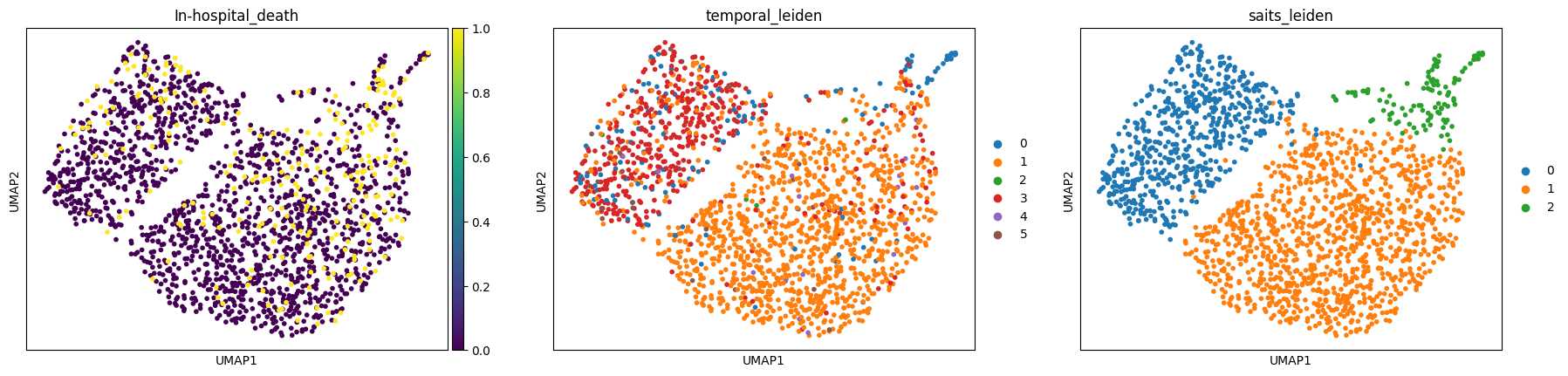
Comparing the unsupervised temporal-statistic clustering with the supervised SAITS-based clustering reveals how much additional structure the model captures from the mortality signal.

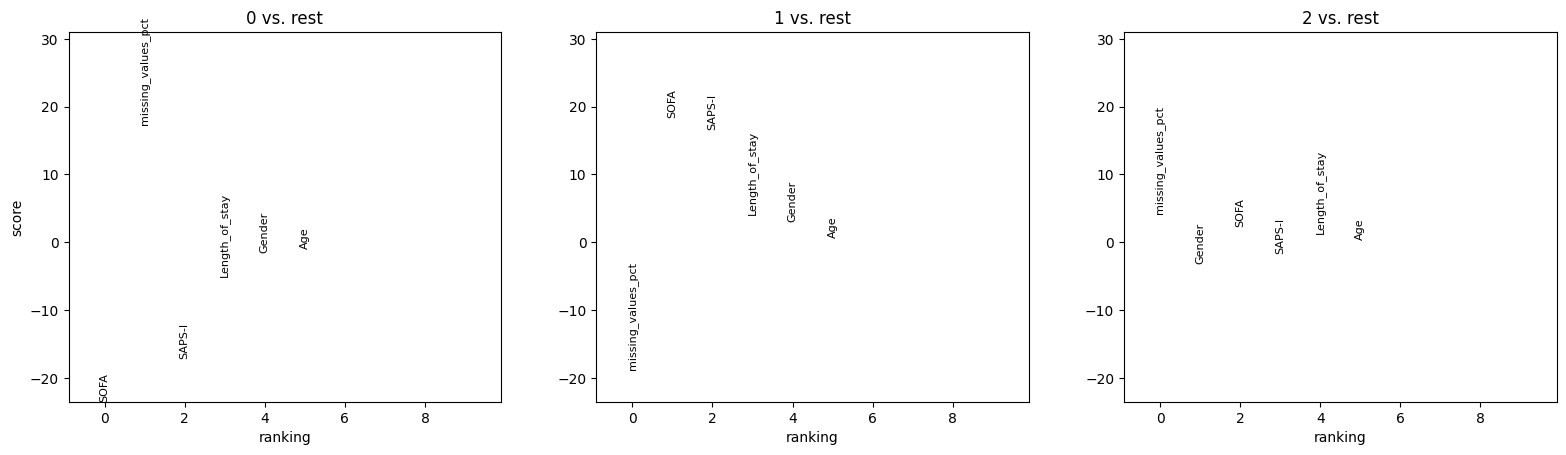
ep.tl.rank_features_groups(
    edata_test,
    field_to_rank="obs",
    columns_to_rank={"obs_names": ["Age", "Gender", "SAPS-I", "SOFA", "Length_of_stay", "missing_values_pct"]},
    groupby="saits_leiden",
    key_added="rank_features_groups",
)
ep.pl.rank_features_groups(edata_test, key="rank_features_groups", n_features=10, show=False);

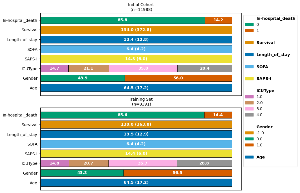
Cohort Tracking Summary

Finally, we can visualize how the cohort changed throughout the full analysis pipeline using the CohortTracker we initialized earlier.

ct.plot_cohort_barplot(
    subfigure_title=True,
    show=True,
    fontsize=10,
    subplots_kwargs={
        "figsize": (9, 8),
        "gridspec_kw": {"wspace": 0.15, "hspace": 0.15},
    },
)