
MIMIC-II IAC Causal Inference#
This tutorial continues the exploration the MIMIC-II IAC dataset using causal inference methods. The dataset was created for the purpose of a case study in the book: Secondary Analysis of Electronic Health Records, published by Springer in 2016. In particular, the dataset was used throughout Chapter 16 (Data Analysis) by Raffa J. et al. to investigate the effectiveness of indwelling arterial catheters in hemodynamically stable patients with respiratory failure for mortality outcomes. The dataset is derived from MIMIC-II, the publicly-accessible critical care database. It contains summary clinical data and outcomes for 1,776 patients.
References:
[1] https://github.com/py-why/dowhy
[2] https://www.pywhy.org/dowhy/
[3] https://arxiv.org/abs/2011.04216
[4] https://physionet.org/content/mimic2-iaccd/1.0/
Environment Setup#
# pip install ehrapy[causal]
from bokeh.io import output_notebook
from bokeh.resources import INLINE

output_notebook(resources=INLINE)
import warnings

warnings.filterwarnings("ignore")

import ehrapy as ep
import ehrdata as ed
import graphviz
from IPython.display import display


MIMIC-II dataset preparation#
Let’s load the MIMIC-II dataset, and using ehrapy encode categorical variables with a one-hot encoding.
edata = ed.dt.mimic_2()
ed.infer_feature_types(edata)
edata = ep.pp.encode(edata, autodetect=True)
! Features 'aline_flg', 'gender_num', 'service_num', 'day_icu_intime_num', 'hour_icu_intime', 'hosp_exp_flg', 'icu_exp_flg', 'day_28_flg', 'censor_flg', 'sepsis_flg', 'chf_flg', 'afib_flg', 'renal_flg', 'liver_flg', 'copd_flg', 'cad_flg', 'stroke_flg', 'mal_flg', 'resp_flg' were detected as categorical features stored numerically. Adjust using `ed.replace_feature_types` if needed.
 Detected feature types for EHRData object with 1776 obs and 46 vars
╠══ 📅 Date features
╠══ 📐 Numerical features
║   ╠══ abg_count
║   ╠══ age
║   ╠══ bmi
║   ╠══ bun_first
║   ╠══ chloride_first
║   ╠══ creatinine_first
║   ╠══ hgb_first
║   ╠══ hospital_los_day
║   ╠══ hr_1st
║   ╠══ icu_los_day
║   ╠══ iv_day_1
║   ╠══ map_1st
║   ╠══ mort_day_censored
║   ╠══ pco2_first
║   ╠══ platelet_first
║   ╠══ po2_first
║   ╠══ potassium_first
║   ╠══ sapsi_first
║   ╠══ sodium_first
║   ╠══ sofa_first
║   ╠══ spo2_1st
║   ╠══ tco2_first
║   ╠══ temp_1st
║   ╠══ wbc_first
║   ╚══ weight_first
╚══ 🗂️ Categorical features
    ╠══ afib_flg (2 categories)
    ╠══ aline_flg (2 categories)
    ╠══ cad_flg (2 categories)
    ╠══ censor_flg (2 categories)
    ╠══ chf_flg (2 categories)
    ╠══ copd_flg (2 categories)
    ╠══ day_28_flg (2 categories)
    ╠══ day_icu_intime (7 categories)
    ╠══ day_icu_intime_num (7 categories)
    ╠══ gender_num (2 categories)
    ╠══ hosp_exp_flg (2 categories)
    ╠══ hour_icu_intime (24 categories)
    ╠══ icu_exp_flg (2 categories)
    ╠══ liver_flg (2 categories)
    ╠══ mal_flg (2 categories)
    ╠══ renal_flg (2 categories)
    ╠══ resp_flg (2 categories)
    ╠══ sepsis_flg (1 categories)
    ╠══ service_num (2 categories)
    ╠══ service_unit (3 categories)
    ╚══ stroke_flg (2 categories)
The MIMIC-II dataset has 1776 patients as described above with 46 features.
edata
EHRData object with n_obs × n_vars = 1776 × 54
    obs: 'service_unit', 'day_icu_intime'
    var: 'feature_type', 'unencoded_var_names', 'encoding_mode'
    layers: 'original'
    shape of .X: (1776, 54)
Causal Inference on the MIMIC-II dataset#
In the background, ehrapy uses the dowhy package to enable effortless causal inference on electronic health records (EHR). Any dowhy analysis is structured into 3 steps:
Formulate causal questions
Estimate causal effects
Perform refutation tests.
Before manually specifying the causal graph, it is useful to get an overview of the statistical dependencies between variables in the dataset. While statistical dependence does not imply causation, it can guide the construction of the directed acylic graph by highlighting which variables are likely related and therefore worth considering as connected nodes.
Note that this visualization is purely exploratory. The causal graph below encodes domain knowledge and assumptions about directionality that go beyond what statistical dependencies alone can tell us.
ep.pl.variable_dependencies(edata, layer="original")
Causal Graph#
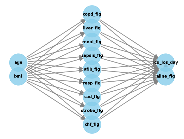
The causal graph is a directed acyclic graph (DAG) that represents the causal relationships between the variables in the dataset. Here, we create it by manually writing out the connections between the variables. Other options would be the GML or DOT graph format. Furthermore, you can use graphical tools like DAGitty to construct the graph. You can export the graph string that it generates. The graph string is very close to the DOT format: just rename dag to digraph, remove newlines and add a semicolon after every line, to convert it to the DOT format and input to DoWhy.
Assumptions:#
both age and overweight increase your risk for medical problems
having a lot of problems makes you more likely to die in the hospital
having a lot of problems influences your likelihood of getting an IAC
having an IAC influences your likelihood of dying in the hospital
causal_graph = """digraph {
aline_flg[label="Indwelling arterial catheters used"];
icu_los_day[label="Days in ICU"];

age -> sepsis_flg;
age -> chf_flg;
age -> afib_flg;
age -> renal_flg;
age -> liver_flg;
age -> copd_flg;
age -> cad_flg;
age -> stroke_flg;
age -> resp_flg;
bmi -> sepsis_flg;
bmi -> chf_flg;
bmi -> afib_flg;
bmi -> renal_flg;
bmi -> liver_flg;
bmi -> copd_flg;
bmi -> cad_flg;
bmi -> stroke_flg;
bmi -> resp_flg;
sepsis_flg -> aline_flg;
chf_flg -> aline_flg;
afib_flg -> aline_flg;
renal_flg -> aline_flg;
liver_flg -> aline_flg;
copd_flg -> aline_flg;
cad_flg -> aline_flg;
stroke_flg -> aline_flg;
resp_flg -> aline_flg;
sepsis_flg -> icu_los_day;
chf_flg -> icu_los_day;
afib_flg -> icu_los_day;
renal_flg -> icu_los_day;
liver_flg -> icu_los_day;
copd_flg -> icu_los_day;
cad_flg -> icu_los_day;
stroke_flg -> icu_los_day;
resp_flg -> icu_los_day;
aline_flg -> icu_los_day;
}"""

g = graphviz.Source(causal_graph)
display(g)

Causal inference#
This graph can now be fed into the causal_inference() method. Furthermore, we have to specify an estimation_method. For now, we will use backdoor.linear_regression.
Please refer to this example notebook and the official dowhy documentation for more information on the different estimation methods.
ep.tl.causal_inference(
    edata=edata,
    graph=causal_graph,
    treatment="aline_flg",
    outcome="icu_los_day",
    estimation_method="backdoor.linear_regression",
)
As we can see, the model returns a summary of the identified causal effect and the refutation results. The placebo_treatment_refuter failed in this case because our intervention variable is binary. By default, all 6 potential refutation methods are run, but the user can also specify to only use a subset of them.
ep.tl.causal_inference(
    edata=edata,
    graph=causal_graph,
    treatment="aline_flg",
    outcome="icu_los_day",
    estimation_method="backdoor.linear_regression",
    refute_methods=[
        "placebo_treatment_refuter",
        "random_common_cause",
        "data_subset_refuter",
        "add_unobserved_common_cause",
        "bootstrap_refuter",
        "dummy_outcome_refuter",
    ],
)
By default, we are hiding a lot of the default dowhy output for clarity. However, it is possible to nontheless display it.
ep.tl.causal_inference(
    edata=edata,
    graph=causal_graph,
    treatment="aline_flg",
    outcome="icu_los_day",
    estimation_method="backdoor.linear_regression",
    refute_methods=[
        # "placebo_treatment_refuter",  # we know it'll fail
        "random_common_cause",
        "data_subset_refuter",
        "add_unobserved_common_cause",
        "bootstrap_refuter",
        "dummy_outcome_refuter",
    ],
    print_causal_estimate=True,
    print_summary=False,
)
Plotting#
Furthermore, the causal_inference() function can generate several plots, if desired. It’s for example possible to output the causal graph …
ep.tl.causal_inference(
    edata=edata,
    graph=causal_graph,
    treatment="aline_flg",
    outcome="icu_los_day",
    estimation_method="backdoor.linear_regression",
    refute_methods=[
        # "placebo_treatment_refuter",  # we know it'll fail
        "random_common_cause",
        "data_subset_refuter",
        "add_unobserved_common_cause",
        "dummy_outcome_refuter",
    ],
    print_causal_estimate=False,
    print_summary=False,
    show_graph=True,
)
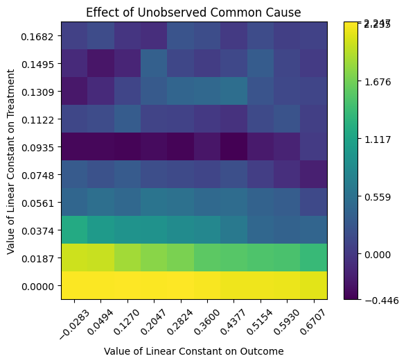
… or the graph generated by the add_unobserved_common_cause refutation method.
ep.tl.causal_inference(
    edata=edata,
    graph=causal_graph,
    treatment="aline_flg",
    outcome="icu_los_day",
    estimation_method="backdoor.linear_regression",
    refute_methods=[
        # "placebo_treatment_refuter",  # we know it'll fail
        "random_common_cause",
        "data_subset_refuter",
        "add_unobserved_common_cause",
        "dummy_outcome_refuter",
    ],
    print_causal_estimate=False,
    print_summary=False,
    show_graph=False,
    show_refute_plots=True,
)
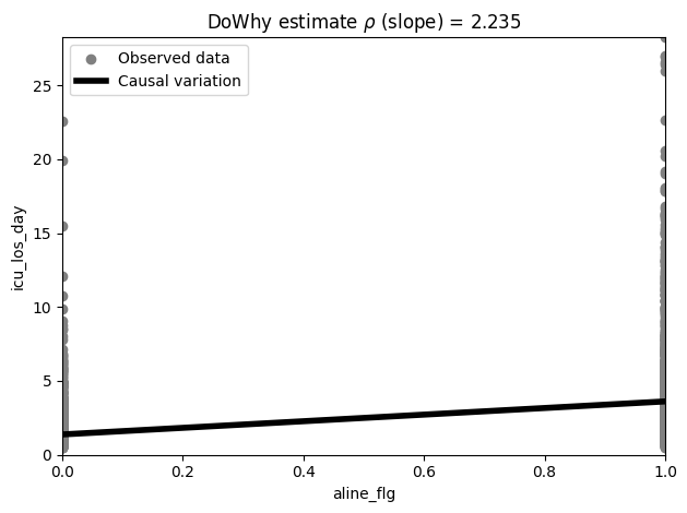
In the process of performing the causal dowhy analysis, an estimator is created which we can query from the model and then visualise.
estimate = ep.tl.causal_inference(
    edata=edata,
    graph=causal_graph,
    treatment="aline_flg",
    outcome="icu_los_day",
    estimation_method="backdoor.linear_regression",
    refute_methods=[
        # "placebo_treatment_refuter",  # we know it'll fail
        "random_common_cause",
        "data_subset_refuter",
        "add_unobserved_common_cause",
        "bootstrap_refuter",
        "dummy_outcome_refuter",
    ],
    print_causal_estimate=False,
    print_summary=False,
    show_graph=False,
    show_refute_plots=False,
    return_as="estimate",
)
ep.pl.causal_effect(estimate)
<Axes: title={'center': 'DoWhy estimate $\\rho$ (slope) = 2.235'}, xlabel='aline_flg', ylabel='icu_los_day'>
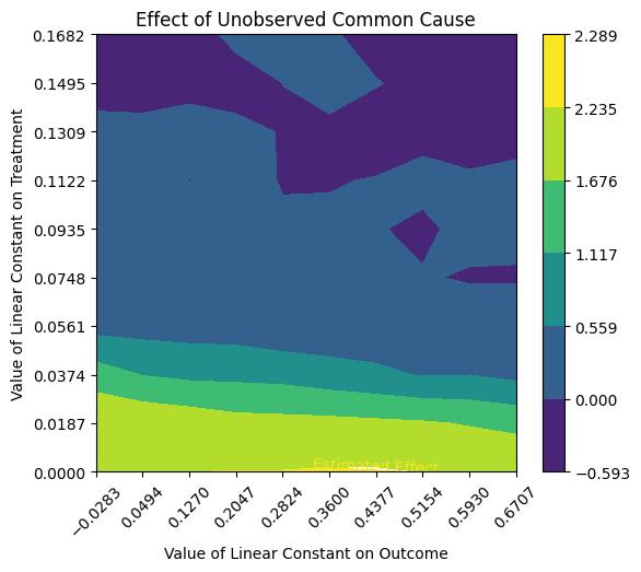
Advanced options#
Within dowhy, the user can specify several arguments for identification, estimation and refutation. These arguments can also be passed directly to the respective functions through the identify_kwargs, estimate_kwargs and refute_kwarg of causal_inference().
estimate = ep.tl.causal_inference(
    edata=edata,
    graph=causal_graph,
    treatment="aline_flg",
    outcome="icu_los_day",
    estimation_method="backdoor.linear_regression",
    refute_methods=[
        # "placebo_treatment_refuter",  # we know it'll fail
        "random_common_cause",
        "data_subset_refuter",
        "add_unobserved_common_cause",
        "bootstrap_refuter",
        "dummy_outcome_refuter",
    ],
    print_causal_estimate=True,
    print_summary=True,
    show_graph=False,
    show_refute_plots="contour",
    return_as="estimate",
    identify_kwargs={"proceed_when_unidentifiable": True},
    estimate_kwargs={"target_units": "days"},
    refute_kwargs={"random_seed": 5},
)
*** Causal Estimate ***

## Identified estimand
Estimand type: EstimandType.NONPARAMETRIC_ATE

### Estimand : 1
Estimand name: backdoor
Estimand expression:
     d                                                                         ↪
────────────(E[icu_los_day|stroke_flg,chf_flg,cad_flg,resp_flg,sepsis_flg,afib ↪
d[aline_flg]                                                                   ↪

↪
↪ _flg,renal_flg,liver_flg,copd_flg])
↪
Estimand assumption 1, Unconfoundedness: If U→{aline_flg} and U→icu_los_day then P(icu_los_day|aline_flg,stroke_flg,chf_flg,cad_flg,resp_flg,sepsis_flg,afib_flg,renal_flg,liver_flg,copd_flg,U) = P(icu_los_day|aline_flg,stroke_flg,chf_flg,cad_flg,resp_flg,sepsis_flg,afib_flg,renal_flg,liver_flg,copd_flg)

## Realized estimand
b: icu_los_day~aline_flg+stroke_flg+chf_flg+cad_flg+resp_flg+sepsis_flg+afib_flg+renal_flg+liver_flg+copd_flg
Target units: days

## Estimate
Mean value: 2.2348813091683177

Causal inference results for treatment variable 'aline_flg' and outcome variable 'icu_los_day':
└- Increasing the treatment variable(s) [aline_flg] from 0 to 1 causes an increase of 2.2348813091683177 in the expected value of the outcome [['icu_los_day']], over the data distribution/population represented by the dataset.

Refutation results
├-Refute: Add a random common cause
|    ├- Estimated effect: 2.23
|    ├- New effect: 2.235
|    ├- p-value: 0.475
|    └- Test significance: 2.23
├-Refute: Use a subset of data
|    ├- Estimated effect: 2.23
|    ├- New effect: 2.235
|    ├- p-value: 0.499
|    └- Test significance: 2.23
├-Refute: Add an Unobserved Common Cause
|    ├- Estimated effect: 2.23
|    ├- New effect: -0.59, 2.29
|    ├- p-value: Not applicable
|    └- Test significance: 2.23
├-Refute: Bootstrap Sample Dataset
|    ├- Estimated effect: 2.23
|    ├- New effect: 2.226
|    ├- p-value: 0.473
|    └- Test significance: 2.23
└-Refute: Use a Dummy Outcome
     ├- Estimated effect: 0.00
     ├- New effect: -0.004
     ├- p-value: 0.466
     └- Test significance: 0.00