ehrapy.plot.kmf#
- ehrapy.plot.kmf(kmfs=None, ci_alpha=None, ci_force_lines=None, ci_show=None, ci_legend=None, at_risk_counts=None, color=None, grid=False, xlim=None, ylim=None, xlabel=None, ylabel=None, figsize=None, show=None, title=None)[source]#
Plots a pretty figure of the Fitted KaplanMeierFitter model
See https://lifelines.readthedocs.io/en/latest/fitters/univariate/KaplanMeierFitter.html
- Parameters:
kmfs (
Optional[Sequence[KaplanMeierFitter]]) – Iterables of fitted KaplanMeierFitter objects.ci_alpha (
Optional[list[float]]) – The transparency level of the confidence interval. If more than one kmfs, this should be a list. Defaults to 0.3.ci_force_lines (
Optional[list[bool]]) – Force the confidence intervals to be line plots (versus default shaded areas). If more than one kmfs, this should be a list. Defaults to False .ci_show (
Optional[list[bool]]) – Show confidence intervals. If more than one kmfs, this should be a list. Defaults to True .ci_legend (
Optional[list[bool]]) – If ci_force_lines is True, this is a boolean flag to add the lines’ labels to the legend. If more than one kmfs, this should be a list. Defaults to False .at_risk_counts (
Optional[list[bool]]) – Show group sizes at time points. If more than one kmfs, this should be a list. Defaults to False.color (
Optional[list[str]]) – List of colors for each kmf. If more than one kmfs, this should be a list.xlim (
Optional[tuple[float,float]]) – Set the x-axis view limits.ylim (
Optional[tuple[float,float]]) – Set the y-axis view limits.figsize (
Optional[tuple[float,float]]) – Width, height in inches. Defaults to None .
Examples
>>> import ehrapy as ep
>>> import numpy as np
>>> adata = ep.dt.mimic_2(encoded=False)
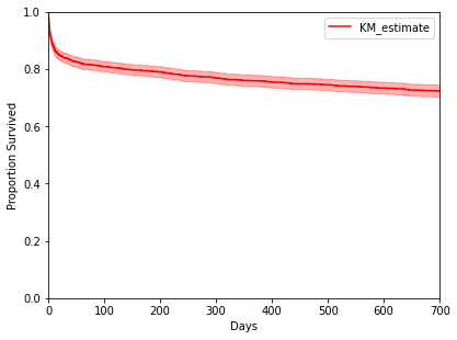
# Because in MIMIC-II database, censor_fl is censored or death (binary: 0 = death, 1 = censored). # While in KaplanMeierFitter, event_observed is True if the the death was observed, False if the event was lost (right-censored). # So we need to flip censor_fl when pass censor_fl to KaplanMeierFitter
>>> adata[:, ['censor_flg']].X = np.where(adata[:, ['censor_flg']].X == 0, 1, 0)
>>> kmf = ep.tl.kmf(adata[:, ['mort_day_censored']].X, adata[:, ['censor_flg']].X)
>>> ep.pl.kmf([kmf], color=['r'], xlim=[0, 700], ylim=[0, 1], xlabel="Days", ylabel="Proportion Survived", show=True)
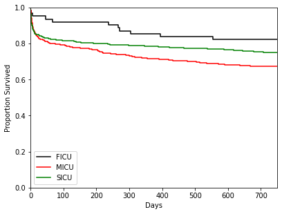
>>> T = adata[:, ['mort_day_censored']].X
>>> E = adata[:, ['censor_flg']].X
>>> groups = adata[:, ['service_unit']].X
>>> ix1 = (groups == 'FICU')
>>> ix2 = (groups == 'MICU')
>>> ix3 = (groups == 'SICU')
>>> kmf_1 = ep.tl.kmf(T[ix1], E[ix1], label='FICU')
>>> kmf_2 = ep.tl.kmf(T[ix2], E[ix2], label='MICU')
>>> kmf_3 = ep.tl.kmf(T[ix3], E[ix3], label='SICU')
>>> ep.pl.kmf([kmf_1, kmf_2, kmf_3], ci_show=[False,False,False], color=['k','r', 'g'],
>>>           xlim=[0, 750], ylim=[0, 1], xlabel="Days", ylabel="Proportion Survived")