Longitudinal Data Analysis: SAITS on the PhysioNet Challenge Dataset

This comprehensive tutorial demonstrates advanced machine learning workflows on clinical time series data using:

• EHRData for structured longitudinal clinical data handling

• PyPOTS for state-of-the-art time series classification on partially-observed time series

• ehrapy for comprehensive data and representation exploration and visualization

• PhysioNet 2012 Challenge dataset for in-hospital mortality prediction

Note

If you’re new to ehrapy and ehrdata, we strongly recommend to read Getting started with ehrdata and Introduction to ehrapy.

Installation and Setup

# pip install pypots

Imports

import os
import warnings

warnings.filterwarnings("ignore")

# PyPOTS requires this for scipy compatibility
os.environ["SCIPY_ARRAY_API"] = "1"

import ehrapy as ep
import ehrdata as ed
import matplotlib.pyplot as plt
import numpy as np
import seaborn as sns
import torch
from pypots.classification import SAITS
from sklearn.metrics import accuracy_score, auc, confusion_matrix, f1_score, precision_recall_curve, roc_auc_score
from sklearn.model_selection import train_test_split

# Set random seeds for reproducibility
torch.manual_seed(42);

Load PhysioNet 2012 Dataset

The Physionet 2012 challenge dataset is one of the built-in, ready-to-use datasets of ehrdata and can be loaded with one line of code:

edata = ed.dt.physionet2012(layer="tem_data")
edata

View of EHRData object with n_obs × n_vars × n_t = 11988 × 37 × 48
    obs: 'set', 'Age', 'Gender', 'Height', 'ICUType', 'SAPS-I', 'SOFA', 'Length_of_stay', 'Survival', 'In-hospital_death'
    var: 'Parameter'
    tem: '0', '1', '2', '3', '4', '5', '6', '7', '8', '9', '10', '11', '12', '13', '14', '15', '16', '17', '18', '19', '20', '21', '22', '23', '24', '25', '26', '27', '28', '29', '30', '31', '32', '33', '34', '35', '36', '37', '38', '39', '40', '41', '42', '43', '44', '45', '46', '47'
    layers: 'tem_data'
    shape of .tem_data: (11988, 37, 48)

print(f"Dataset shape: {edata.shape}")
print(f"Number of patients: {edata.n_obs}")
print(f"Number of longitudinalvariables: {edata.n_vars}")
print(f"Number of time points: {edata.n_t}")
print(f"\nObservation metadata columns: {list(edata.obs.columns)}")
print(f"\nVariable names: {list(edata.var_names[:10])}...")  # Show first 10

Dataset shape: (11988, 37, 48)
Number of patients: 11988
Number of longitudinalvariables: 37
Number of time points: 48

Observation metadata columns: ['set', 'Age', 'Gender', 'Height', 'ICUType', 'SAPS-I', 'SOFA', 'Length_of_stay', 'Survival', 'In-hospital_death']

Variable names: ['ALP', 'ALT', 'AST', 'Albumin', 'BUN', 'Bilirubin', 'Cholesterol', 'Creatinine', 'DiasABP', 'FiO2']...

Lets inspect the static data:

edata.obs.head()

	set	Age	Gender	Height	ICUType	SAPS-I	SOFA	Length_of_stay	Survival	In-hospital_death
RecordID
132539	set-a	54.0	0.0	-1.0	4.0	6	1	5	-1	0
132540	set-a	76.0	1.0	175.3	2.0	16	8	8	-1	0
132541	set-a	44.0	0.0	-1.0	3.0	21	11	19	-1	0
132543	set-a	68.0	1.0	180.3	3.0	7	1	9	575	0
132545	set-a	88.0	0.0	-1.0	3.0	17	2	4	918	0

And have a look at the dynamic variables:

ed.infer_feature_types(edata, layer="tem_data")

! Feature  was detected as categorical features stored numerically.Please verify and adjust if necessary using `ed.replace_feature_types`.

 Detected feature types for EHRData object with 11988 obs and 37 vars
╠══ 📅 Date features
╠══ 📐 Numerical features
║   ╠══ ALP
║   ╠══ ALT
║   ╠══ AST
║   ╠══ Albumin
║   ╠══ BUN
║   ╠══ Bilirubin
║   ╠══ Cholesterol
║   ╠══ Creatinine
║   ╠══ DiasABP
║   ╠══ FiO2
║   ╠══ GCS
║   ╠══ Glucose
║   ╠══ HCO3
║   ╠══ HCT
║   ╠══ HR
║   ╠══ K
║   ╠══ Lactate
║   ╠══ MAP
║   ╠══ MechVent
║   ╠══ Mg
║   ╠══ NIDiasABP
║   ╠══ NIMAP
║   ╠══ NISysABP
║   ╠══ Na
║   ╠══ PaCO2
║   ╠══ PaO2
║   ╠══ Platelets
║   ╠══ RespRate
║   ╠══ SaO2
║   ╠══ SysABP
║   ╠══ Temp
║   ╠══ TroponinI
║   ╠══ TroponinT
║   ╠══ Urine
║   ╠══ WBC
║   ╠══ Weight
║   ╚══ pH
╚══ 🗂️ Categorical features

Exploratory Data Analysis

Comprehensive Data Inspection with ehrapy

We’ll use ehrapy’s powerful inspection tools to understand our cohort and data quality.

Quality control metrics with ehrapy

Before diving into cohort tracking and missing value analysis, we compute quality control (QC) metrics using ep.pp.qc_metrics. This adds missing-value statistics and summary statistics (mean, median, std, etc.) to edata.obs and edata.var, which supports downstream filtering and interpretation. For longitudinal data we use the tem_data layer.

# Compute QC metrics on the temporal data layer
# Adds missing_values_abs, missing_values_pct, entropy_of_missingness to obs/var
# plus summary stats (mean, median, std, min, max) to var
obs_qc, var_qc = ep.pp.qc_metrics(edata, layer="tem_data")

# Show a preview of observation- and variable-level metrics
print("Observation-level QC metrics (first 5 rows):")
display(obs_qc.head())

print("\nVariable-level QC metrics (first 10 rows):")
display(var_qc)

Observation-level QC metrics (first 5 rows):

	missing_values_abs	missing_values_pct	entropy_of_missingness	unique_values_abs	unique_values_ratio
RecordID
132539	1516	85.360360	0.600748	NaN	NaN
132540	1375	77.421171	0.770597	NaN	NaN
132541	1383	77.871622	0.762505	NaN	NaN
132543	1418	79.842342	0.725070	NaN	NaN
132545	1472	82.882883	0.660377	NaN	NaN

Variable-level QC metrics (first 10 rows):

	missing_values_abs	missing_values_pct	entropy_of_missingness	unique_values_abs	unique_values_ratio	coefficient_of_variation	is_constant	constant_variable_ratio	range_ratio	mean	median	standard_deviation	min	max	iqr_outliers
Parameter
ALP	565999	98.362077	0.120597	NaN	NaN	1.458623	0.0	2.702703	3901.207763	120.142281	82.00	175.242311	8.00	4695.00	True
ALT	565729	98.315155	0.123359	NaN	NaN	3.123187	0.0	2.702703	4661.914393	362.919577	42.00	1133.465814	1.00	16920.00	True
AST	565728	98.314982	0.123370	NaN	NaN	3.266529	0.0	2.702703	7207.158151	504.997937	62.00	1649.590278	4.00	36400.00	True
Albumin	568184	98.741797	0.097461	NaN	NaN	0.225510	0.0	2.702703	148.754802	2.890663	2.90	0.651872	1.00	5.30	True
BUN	533750	92.757688	0.374902	NaN	NaN	0.831778	0.0	2.702703	769.177905	27.171867	20.00	22.600949	0.00	209.00	True
Bilirubin	565631	98.298125	0.124357	NaN	NaN	2.014253	0.0	2.702703	2890.170303	2.864883	0.90	5.770600	0.00	82.80	True
Cholesterol	574430	99.827258	0.018343	NaN	NaN	0.285582	0.0	2.702703	214.539768	155.682093	153.00	44.460024	28.00	362.00	True
Creatinine	533561	92.724843	0.376109	NaN	NaN	1.052263	0.0	2.702703	1493.335020	1.473213	1.00	1.550207	0.10	22.10	True
DiasABP	263572	45.804833	0.994916	NaN	NaN	0.219552	0.0	2.702703	458.459459	59.547250	58.00	13.073717	-1.00	272.00	True
FiO2	485065	84.296971	0.627158	NaN	NaN	0.347687	0.0	2.702703	145.954334	0.541265	0.50	0.188191	0.21	1.00	True
GCS	390948	67.940858	0.905023	NaN	NaN	0.349804	0.0	2.702703	105.123165	11.415181	13.00	3.993081	3.00	15.00	False
Glucose	536149	93.174598	0.359374	NaN	NaN	0.461591	0.0	2.702703	1123.930841	140.844965	127.00	65.012700	8.00	1591.00	True
HCO3	534635	92.911488	0.369218	NaN	NaN	0.203925	0.0	2.702703	202.980067	23.154983	23.00	4.721876	5.00	52.00	True
HCT	520731	90.495183	0.453099	NaN	NaN	0.162944	0.0	2.702703	185.066161	30.691727	30.20	5.001046	5.00	61.80	True
HR	56315	9.786696	0.462197	NaN	NaN	0.206184	0.0	2.702703	346.358382	86.615487	86.00	17.858740	0.00	300.00	True
K	531760	92.411856	0.387498	NaN	NaN	0.164904	0.0	2.702703	518.328873	4.128653	4.00	0.680830	1.50	22.90	True
Lactate	551734	95.883036	0.247629	NaN	NaN	0.868414	0.0	2.702703	1049.155999	2.954756	2.10	2.565953	0.00	31.00	True
MAP	265352	46.114170	0.995639	NaN	NaN	0.204718	0.0	2.702703	372.496691	80.269169	78.00	16.432571	0.00	299.00	True
MechVent	488672	84.923813	0.611744	NaN	NaN	0.000000	1.0	2.702703	0.000000	1.000000	1.00	0.000000	1.00	1.00	False
Mg	534582	92.902277	0.369560	NaN	NaN	0.255141	0.0	2.702703	1853.313572	2.023403	2.00	0.516253	0.00	37.50	True
NIDiasABP	333319	57.925808	0.981798	NaN	NaN	0.260584	0.0	2.702703	310.174927	58.354169	57.00	15.206178	-1.00	180.00	True
NIMAP	336656	58.505728	0.979023	NaN	NaN	0.194690	0.0	2.702703	294.729866	77.358974	76.00	15.061055	0.00	228.00	True
NISysABP	333102	57.888096	0.981971	NaN	NaN	0.187413	0.0	2.702703	250.653579	119.687100	117.00	22.430955	0.00	300.00	True
Na	534543	92.895500	0.369811	NaN	NaN	0.037481	0.0	2.702703	58.948188	139.105208	139.00	5.213751	98.00	180.00	True
PaCO2	509020	88.459988	0.515992	NaN	NaN	0.225958	0.0	2.702703	247.572030	40.392285	39.00	9.126968	0.00	100.00	True
PaO2	509141	88.481016	0.515374	NaN	NaN	0.579941	0.0	2.702703	338.878616	147.545456	121.00	85.567716	0.00	500.00	True
Platelets	533013	92.629609	0.379596	NaN	NaN	0.563801	0.0	2.702703	1203.967210	189.955339	172.00	107.097081	5.00	2292.00	True
RespRate	436953	75.935832	0.796106	NaN	NaN	0.280113	0.0	2.702703	510.486708	19.589149	19.00	5.487177	0.00	100.00	True
SaO2	552318	95.984526	0.243001	NaN	NaN	0.036279	0.0	2.702703	103.423634	96.689699	97.00	3.507824	0.00	100.00	True
SysABP	263549	45.800836	0.994906	NaN	NaN	0.199785	0.0	2.702703	237.713669	119.892138	118.00	23.952596	0.00	285.00	True
Temp	361770	62.870162	0.951664	NaN	NaN	0.038446	0.0	2.702703	161.813111	37.079814	37.10	1.425589	-17.80	42.20	True
TroponinI	574249	99.795803	0.021190	NaN	NaN	1.335988	0.0	2.702703	602.895141	8.210383	3.30	10.968970	0.10	49.60	True
TroponinT	569176	98.914192	0.086429	NaN	NaN	2.371901	0.0	2.702703	2545.321914	1.174704	0.18	2.786282	0.01	29.91	True
Urine	176761	30.718392	0.889896	NaN	NaN	1.368211	0.0	2.702703	9489.392139	115.918911	70.00	158.601586	0.00	11000.00	True
WBC	536674	93.265835	0.355924	NaN	NaN	0.809768	0.0	2.702703	4082.121674	12.934450	11.50	10.473903	0.00	528.00	True
Weight	271296	47.147147	0.997650	NaN	NaN	0.302450	0.0	2.702703	569.253256	83.091312	80.00	25.130950	-1.00	472.00	True
pH	504442	87.664401	0.538931	NaN	NaN	0.675547	0.0	2.702703	10051.342566	7.312456	7.38	4.939904	0.00	735.00	True

We can see at a glance

• what percentage of measurements are available on an observation (person) level

• what percentage of measurements are available on a variable level

For the persons, we see from the sample of the first 5 individuals that the missing value percentage, or in other words the monitoring intensity, can vary.

Further, for the variables, information such as summary statistics such as the mean, and whether outliers are present.

Remember we consider values measured in hourly intervals for 48 hours;

Here, we note that the basic physiological measurements such as DiasABP, HR, MAP, NIDiasABP, NIMAP, NISysABP, SysABP, Urine, and Weight are most frequently recorded.

More specific measurements such as for instance WBC and TroponinI are less frequently measured.

Cohort Tracking with CohortTracker

Let us examine the static information of the cohort in a bit more detail. This can be reported as a table using the tableone package, or visually using ehrapy’s CohortTracker, which will be able to display further information at the end of the notebook.

from tableone import TableOne

tableone = TableOne(edata.obs, categorical=["set", "Gender", "ICUType", "In-hospital_death"])
display(tableone)

		Missing	Overall
n			11988
set, n (%)	set-a		3997 (33.3)
	set-b		3993 (33.3)
	set-c		3998 (33.4)
Age, mean (SD)		0	64.5 (17.2)
Gender, n (%)	-1.0		12 (0.1)
	0.0		5259 (43.9)
	1.0		6717 (56.0)
Height, mean (SD)		0	88.2 (86.1)
ICUType, n (%)	1.0		1765 (14.7)
	2.0		2528 (21.1)
	3.0		4287 (35.8)
	4.0		3408 (28.4)
SAPS-I, mean (SD)		0	14.3 (6.0)
SOFA, mean (SD)		0	6.4 (4.2)
Length_of_stay, mean (SD)		0	13.4 (12.8)
Survival, mean (SD)		0	134.0 (372.8)
In-hospital_death, n (%)	0		10281 (85.8)
	1		1707 (14.2)
missing_values_abs, mean (SD)		0	1415.5 (77.3)
missing_values_pct, mean (SD)		0	79.7 (4.4)
entropy_of_missingness, mean (SD)		0	0.7 (0.1)
unique_values_abs, mean (SD)		11988	nan (nan)
unique_values_ratio, mean (SD)		11988	nan (nan)

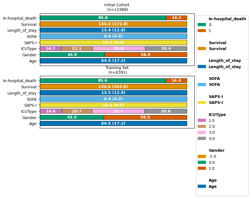
tracking_cols = ["Age", "Gender", "ICUType", "SAPS-I", "SOFA", "Length_of_stay", "Survival", "In-hospital_death"]
categorical_cols = ["Gender", "ICUType", "In-hospital_death"]

ct = ep.tl.CohortTracker(edata, columns=tracking_cols, categorical=categorical_cols)
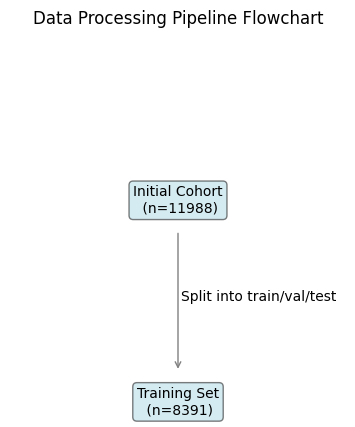
ct(edata, label="Initial Cohort", operations_done="Loaded PhysioNet 2012 dataset")
ct.plot_cohort_barplot()

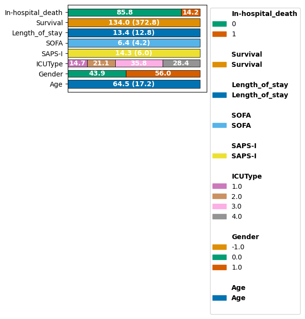
We can observe that on average, patients are 64.5 years old upon ICU entry, with slightly more females (0) than males (1).

Sankey Diagrams for Patient Flow

We can further inspect static variables with a Sankey diagram:

ep.pl.sankey_diagram(
    edata,
    columns=["Gender", "In-hospital_death"],
    title="Patient Flow: Gender to Sepsis Status",
)

Where we can obtain a quick visual queue about e.g. the relation of Gender and In-hospital_death.

Here, there is no immediate indication that these two variables are strongly associated in our cohort.

We can also inspect variables longitudinally for how patients change along the time axis. A Sankey diagram is for categorical variables. Since our time-series data consists of continuous variables, we create a quick example with categorized values.

For this, let us explore the heart rate HR, which we bin for a rough overview into low, normal, high, and missing.

# create a new layer in edata
edata.layers["cat_hr"] = edata.layers["tem_data"].copy()

# fill the HR variable (index 14) with the categorical values
edata.layers["cat_hr"][:, 14, :] = np.where(
    edata.layers["tem_data"][:, 14, :] < 60, 0, edata.layers["cat_hr"][:, 14, :]
)
edata.layers["cat_hr"][:, 14, :] = np.where(
    edata.layers["tem_data"][:, 14, :] >= 100, 2, edata.layers["cat_hr"][:, 14, :]
)
edata.layers["cat_hr"][:, 14, :] = np.where(
    (edata.layers["tem_data"][:, 14, :] >= 60) & (edata.layers["tem_data"][:, 14, :] <= 100),
    1,
    edata.layers["cat_hr"][:, 14, :],
)
edata.layers["cat_hr"][:, 14, :] = np.where(
    np.isnan(edata.layers["tem_data"][:, 14, :]), 3, edata.layers["cat_hr"][:, 14, :]
)

Let’s visualize these HR categories for the first 10 hours:

# plot the Sankey diagram
ep.pl.sankey_diagram_time(
    edata[:, :, :5],
    var_name="HR",
    layer="cat_hr",
    state_labels={0: "Low HR", 1: "Normal HR", 2: "High HR", 3: "Missing HR"},
    width=700,
)

We can see that most patients at hour 0 (leftmost) have no HR measurement. Further, most patients with measured HR display a normal measurement at hour 0.

We can observe that the fraction of patients with no HR measurement at every hour declines as their ICU stay procedes.

Time Series Visualization

For exploring continuous variables across time, lineplots or timeseries plots are more suitable.

Let’s explore for instance a few of the vital parameters for the two first patients:

vital_vars = ["HR", "SaO2", "Temp", "NISysABP", "NIDiasABP", "RespRate"]

ep.pl.timeseries(
    edata[:2],
    layer="tem_data",
    var_names=vital_vars,
)

We can see that the measurements of vital signs can be very irregular, and different for different individuals; While individual 132540 had their HR constantly monitored, no data on their RespRate is available. Individual 132539 on the other hand has HR and RespRate data available, but multiple gaps where none of these values were acquired.

Normalization

As we also can see in the plot above, variables have different scales, which are further arbitrary by the units that is used. To treat features equally in modelling, and to focus on within-feature deviation from “standard” instead of focusing on numeric magnitude, we normalize them. ehrapy offers multiple ways to do so, here we use robust scale norm for all variables.

In rest of notebook, we use normalized data.

edata.layers["norm_data"] = edata.layers["tem_data"].copy()

ep.pp.scale_norm(edata, layer="norm_data")

We add a normalized_imputed layer by filling missing values in the normalized data with 0 using ep.pp.explicit_impute. For z-normalized data, the mean is 0, so replacing missings with 0 is analogous to mean imputation. Ehrapy offers more choices and sophisticated imputation methods (e.g. iterative/model-based) for settings where a simple fill value is not appropriate.

And if we inspect this timeseries plot again:

vital_vars = ["HR", "SaO2", "Temp", "NISysABP", "NIDiasABP", "RespRate"]
ep.pl.timeseries(
    edata[:2],
    layer="norm_data",
    var_names=vital_vars,
)

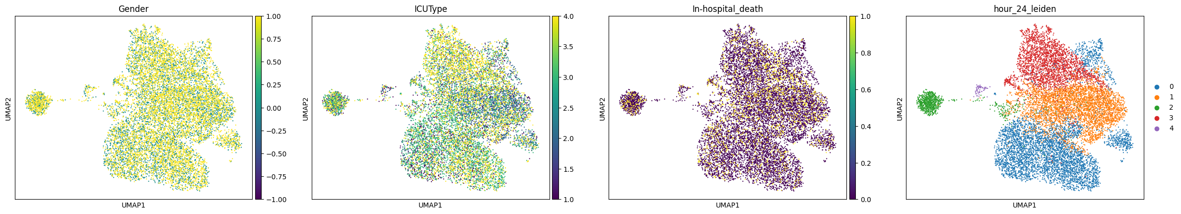
Time-point representations

We build representations at hour 24 and hour 48 by slicing the normalized_imputed layer at those time indices to obtain 2D patient×feature matrices. For each time point we compute a neighborhood graph, and perform Leiden clustering. We can then vizualise the neighborhood graph as a UMAP.

First we need an imputation approach before computing the neighborhood graph; for simplicity, we use here a simple mean imputation strategy. There are exist also other, more sophisticated approaches.

edata.layers["normalized_imputed"] = edata.layers["norm_data"].copy()
ep.pp.simple_impute(edata, strategy="mean", layer="normalized_imputed")

# Representation at hour 24 put into .obsm of edata
edata.obsm["hour_24"] = edata.layers["normalized_imputed"][:, :, 23]

ep.pp.neighbors(edata, n_neighbors=15, use_rep="hour_24", key_added="hour_24_neighbors")
ep.tl.leiden(edata, neighbors_key="hour_24_neighbors", key_added="hour_24_leiden", resolution=0.2)
ep.tl.umap(edata, neighbors_key="hour_24_neighbors")
ep.pl.umap(edata, color=["Gender", "ICUType", "In-hospital_death", "hour_24_leiden"], show=False)

[<Axes: title={'center': 'Gender'}, xlabel='UMAP1', ylabel='UMAP2'>,
 <Axes: title={'center': 'ICUType'}, xlabel='UMAP1', ylabel='UMAP2'>,
 <Axes: title={'center': 'In-hospital_death'}, xlabel='UMAP1', ylabel='UMAP2'>,
 <Axes: title={'center': 'hour_24_leiden'}, xlabel='UMAP1', ylabel='UMAP2'>]

# Representation at hour 24 put into .obsm of edata
edata.obsm["hour_48"] = edata.layers["normalized_imputed"][:, :, 47]

ep.pp.neighbors(edata, n_neighbors=15, use_rep="hour_48", key_added="hour_48_neighbors")
ep.tl.leiden(edata, neighbors_key="hour_48_neighbors", key_added="hour_48_leiden", resolution=0.2)
ep.tl.umap(edata, neighbors_key="hour_48_neighbors")
ep.pl.umap(edata, color=["Gender", "ICUType", "In-hospital_death", "hour_48_leiden"], show=False)

[<Axes: title={'center': 'Gender'}, xlabel='UMAP1', ylabel='UMAP2'>,
 <Axes: title={'center': 'ICUType'}, xlabel='UMAP1', ylabel='UMAP2'>,
 <Axes: title={'center': 'In-hospital_death'}, xlabel='UMAP1', ylabel='UMAP2'>,
 <Axes: title={'center': 'hour_48_leiden'}, xlabel='UMAP1', ylabel='UMAP2'>]

There appears no clear visual substructure in this 2D projection within the patients at hour 24 or 48 with this simple strategy.

Let us also have a look at the unsupervised leiden clustering.

Rank features groups

We identify static features that differ across Leiden clusters using ep.tl.rank_features_groups on the hour-48 representation. This concludes the exploratory section.

ep.tl.rank_features_groups(
    edata,
    field_to_rank="obs",
    columns_to_rank={"obs_names": ["Age", "Gender", "SAPS-I", "SOFA", "Length_of_stay", "missing_values_pct"]},
    groupby="hour_48_leiden",
    key_added="rank_features_groups",
)
ep.pl.rank_features_groups(edata, key="rank_features_groups", n_features=10, show=False)

! Feature  was detected as categorical features stored numerically.Please verify and correct using `ep.ad.replace_feature_types` if necessary.
! Detected no columns that need to be encoded. Leaving passed EHRData/AnnData object unchanged.

[<Axes: title={'center': '0 vs. rest'}, xlabel='ranking', ylabel='score'>,
 <Axes: title={'center': '1 vs. rest'}, xlabel='ranking'>,
 <Axes: title={'center': '2 vs. rest'}, xlabel='ranking'>]

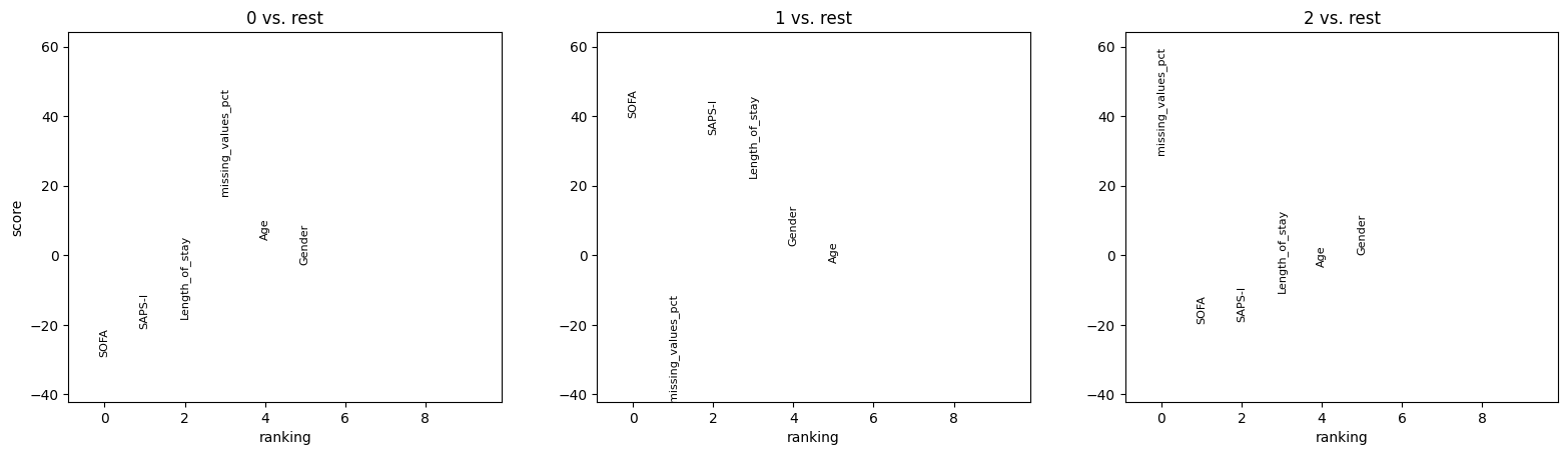
We can observe that the Leiden clustering, defined entirely on dynamic variables at hour 48, subgrouped the patients into a group of low SOFA and SAPS-I score, a group of high SOFA and SAPS-I score, and a group of high missing value frequency.

Machine Learning with SAITS

Now that we’ve comprehensively explored the data, patient representations, and clustering patterns, we’ll build a deep learning model to predict in-hospital mortality using the SAITS architecture from PyPOTS.

SAITS (Self-Attention-based Imputation for Time Series) is designed for classification on partially-observed time series data, making it ideal for clinical applications where missing values are common.

SAITS Model Setup

SAITS (Self-Attention-based Imputation for Time Series) is a powerful model for classification on partially-observed time series. In the PyPOTS implementation, it follows a unified classifier API shared with other models like BRITS, Raindrop, and iTransformer, and uses diagonal masked self-attention (DMSA) to handle missingness patterns.[PyPOTS docs]

Key aspects of the setup:

1. Input format: (X \in \mathbb{R}^{N \times T \times D}) with missing values allowed

2. Unified training API: fit(train_set, val_set) where each set is a dict with keys "X" and "y"

3. Inference via predict() and predict_proba(), returning classification labels and probabilities

We start by splitting the data into training, validation, and test sets.

train_indices = np.arange(len(edata))
train_idx, temp_idx = train_test_split(
    train_indices,
    test_size=0.3,
    random_state=42,
    stratify=edata.obs["SepsisLabel"] if "SepsisLabel" in edata.obs.columns else None,
)
val_idx, test_idx = train_test_split(
    temp_idx,
    test_size=0.5,
    random_state=42,
    stratify=edata.obs.iloc[temp_idx]["SepsisLabel"] if "SepsisLabel" in edata.obs.columns else None,
)

edata_train = edata[train_idx].copy()
edata_val = edata[val_idx].copy()
edata_test = edata[test_idx].copy()

# Track cohort changes
ct(edata_train, label="Training Set", operations_done="Split into train/val/test")

We configure SAITS for PhysioNet 2012 with:

• Sequence length: 48 hourly steps

• Number of features: 37 clinical variables

• Binary classification: in-hospital mortality vs. no in-hospital mortality

• DMSA architecture with 2 layers, d_model=64, n_heads=4 (so d_k=d_v=16)

• Moderate number of epochs and batch size suitable for this dataset

# Initialize SAITS classifier
n_timesteps = edata_train.shape[2]
n_features = edata_train.shape[1]
n_classes = 2  # Binary classification: in-hospital death vs. no in-hospital death

# SAITS architecture: d_model must be divisible by n_heads, d_k = d_model / n_heads
d_model = 64
n_heads = 4
d_k = d_v = d_model // n_heads  # 16

# Initialize SAITS with PyPOTS defaults and reasonable training settings
saits = SAITS(
    n_steps=n_timesteps,
    n_features=n_features,
    n_classes=n_classes,
    # Architecture parameters required by SAITS
    n_layers=2,
    d_model=d_model,
    n_heads=n_heads,
    d_k=d_k,
    d_v=d_v,
    d_ffn=128,
    dropout=0.1,
    attn_dropout=0.1,
    diagonal_attention_mask=True,  # DMSA
    # Training configuration
    epochs=4,
    batch_size=32,
    patience=1,
    device="cuda" if torch.cuda.is_available() else "cpu",
    saving_path="./saits_model",  # Save model checkpoints
)

print(f"\nUsing device: {saits.device}")
print(f"Model initialized with {sum(p.numel() for p in saits.model.parameters())} parameters")

2026-01-28 01:41:41 [INFO]: Using the given device: cpu
2026-01-28 01:41:41 [INFO]: Model files will be saved to ./saits_model/20260128_T014141
2026-01-28 01:41:41 [INFO]: Tensorboard file will be saved to ./saits_model/20260128_T014141/tensorboard
2026-01-28 01:41:41 [INFO]: Using customized CrossEntropy as the training loss function.
2026-01-28 01:41:41 [INFO]: Using customized CrossEntropy as the validation metric function.
2026-01-28 01:41:41 [INFO]: SAITS initialized with the given hyperparameters, the number of trainable parameters: 155,416

Using device: cpu
Model initialized with 155416 parameters

Now, we can train the model

saits.fit(
    train_set={
        "X": edata_train.layers["norm_data"].transpose(0, 2, 1),
        "y": edata_train.obs["In-hospital_death"].values,
    },
    val_set={"X": edata_val.layers["norm_data"].transpose(0, 2, 1), "y": edata_val.obs["In-hospital_death"].values},
)

2026-01-28 01:41:50 [INFO]: Epoch 001 - training loss (CrossEntropy): 0.3638, validation CrossEntropy: 0.3001
2026-01-28 01:41:57 [INFO]: Epoch 002 - training loss (CrossEntropy): 0.3231, validation CrossEntropy: 0.2932
2026-01-28 01:42:05 [INFO]: Epoch 003 - training loss (CrossEntropy): 0.3061, validation CrossEntropy: 0.2890
2026-01-28 01:42:13 [INFO]: Epoch 004 - training loss (CrossEntropy): 0.2961, validation CrossEntropy: 0.3069
2026-01-28 01:42:13 [INFO]: Exceeded the training patience. Terminating the training procedure...
2026-01-28 01:42:13 [INFO]: Finished training. The best model is from epoch#3.
2026-01-28 01:42:13 [INFO]: Saved the model to ./saits_model/20260128_T014141/SAITS.pypots

Model Evaluation

We now evaluate our prediction model using some classical performance reporting metrics.

# Evaluate the trained SAITS classifier on the test set
test_predictions = saits.predict({"X": edata_test.layers["norm_data"].transpose(0, 2, 1)})

test_pred_labels = test_predictions["classification"]
test_pred_proba = test_predictions["classification_proba"]

y_test = edata_test.obs["In-hospital_death"]
# Calculate metrics
roc_auc = roc_auc_score(y_test, test_pred_proba[:, 1])
precision, recall, _ = precision_recall_curve(y_test, test_pred_proba[:, 1])
pr_auc = auc(recall, precision)
f1 = f1_score(y_test, test_pred_labels)
accuracy = accuracy_score(y_test, test_pred_labels)

print("\nTest Set Performance:")
print(f"  ROC-AUC: {roc_auc:.4f}")
print(f"  PR-AUC: {pr_auc:.4f}")
print(f"  F1 Score: {f1:.4f}")
print(f"  Accuracy: {accuracy:.4f}")

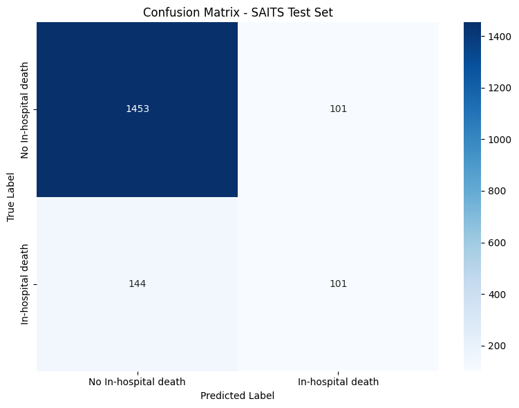
# Confusion matrix
cm = confusion_matrix(y_test, test_pred_labels)
print("\nConfusion Matrix:")
print(f"  True Negatives: {cm[0, 0]}, False Positives: {cm[0, 1]}")
print(f"  False Negatives: {cm[1, 0]}, True Positives: {cm[1, 1]}")

# Visualize confusion matrix
plt.figure(figsize=(8, 6))
sns.heatmap(
    cm,
    annot=True,
    fmt="d",
    cmap="Blues",
    xticklabels=["No In-hospital death", "In-hospital death"],
    yticklabels=["No In-hospital death", "In-hospital death"],
)
plt.title("Confusion Matrix - SAITS Test Set")
plt.ylabel("True Label")
plt.xlabel("Predicted Label")
plt.tight_layout()
plt.show()

Test Set Performance:
  ROC-AUC: 0.8376
  PR-AUC: 0.4841
  F1 Score: 0.4519
  Accuracy: 0.8638

Confusion Matrix:
  True Negatives: 1453, False Positives: 101
  False Negatives: 144, True Positives: 101

# Plot ROC and PR curves
fig, (ax1, ax2) = plt.subplots(1, 2, figsize=(14, 5))

# ROC Curve
from sklearn.metrics import roc_curve

fpr, tpr, _ = roc_curve(y_test, test_pred_proba[:, 1])
ax1.plot(fpr, tpr, label=f"SAITS (AUC = {roc_auc:.3f})", linewidth=2)
ax1.plot([0, 1], [0, 1], "k--", label="Random")
ax1.set_xlabel("False Positive Rate", fontsize=12)
ax1.set_ylabel("True Positive Rate", fontsize=12)
ax1.set_title("ROC Curve", fontsize=14)
ax1.legend(fontsize=11)
ax1.grid(alpha=0.3)

# PR Curve
ax2.plot(recall, precision, label=f"SAITS (AUC = {pr_auc:.3f})", linewidth=2)
baseline = y_test.mean()
ax2.plot([0, 1], [baseline, baseline], "k--", label=f"Baseline ({baseline:.3f})")
ax2.set_xlabel("Recall", fontsize=12)
ax2.set_ylabel("Precision", fontsize=12)
ax2.set_title("Precision-Recall Curve", fontsize=14)
ax2.legend(fontsize=11)
ax2.grid(alpha=0.3)

plt.tight_layout()
plt.show()

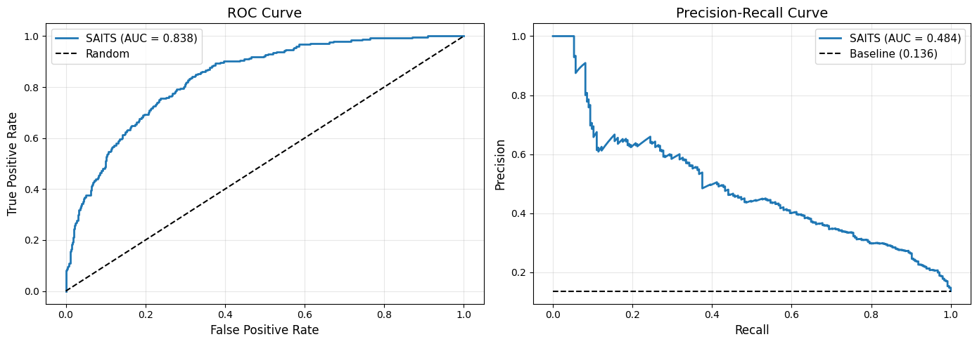
We can already get a rough impression: The label imbalance, much more non-mortal than mortal cases, makes the model lean towards predicting “no In-hospital death” in most cases.

Exploring SAITS Representations

While SAITS is trained in a supervised manner and outputs a label, we can extract representations for patient embeddings.

This is a supervised representation learning approach contrasted with the simple time-based cross-sections from Section 1.2.

# prepare data for PyPOTS' saits backbone
data = edata_test.layers["tem_data"].transpose(0, 2, 1).copy()
missing_mask = np.isnan(data)
data[missing_mask] = 0
data = torch.tensor(data, dtype=torch.float32)

# get the saits embedding
_, _, X_tilde_3, _, _, _ = saits.model.encoder(
    torch.tensor(data, dtype=torch.float32),
    torch.tensor(missing_mask, dtype=torch.float32),
    None,
)

We store the embedding again in the .obsm slot of our EHRData object.

edata_test.obsm["saits_embedding"] = X_tilde_3.mean(dim=1).detach().numpy()

And perform neighborhood graph construction, and subsequent leiden clustering and UMAP computation on this embedding:

ep.pp.neighbors(edata_test, use_rep="saits_embedding", key_added="saits_neighbors", n_neighbors=15)
ep.tl.leiden(edata_test, neighbors_key="saits_neighbors", key_added="saits_leiden", resolution=0.2)
ep.tl.umap(edata_test, neighbors_key="saits_neighbors")

We can visualize this in 2D, and compare also e.g. the leiden clustering from the 48h time cross-section from before with the newly computed leiden clustering on the SAITS embedding.

ep.pl.umap(
    edata_test,
    color=["Gender", "ICUType", "In-hospital_death", "hour_48_leiden", "saits_leiden"],
    title="UMAP: In-hospital_death",
    show=False,
)

WARNING: The title list is shorter than the number of panels. Using 'color' value instead for some plots.
WARNING: The title list is shorter than the number of panels. Using 'color' value instead for some plots.
WARNING: The title list is shorter than the number of panels. Using 'color' value instead for some plots.
WARNING: The title list is shorter than the number of panels. Using 'color' value instead for some plots.

[<Axes: title={'center': 'UMAP: In-hospital_death'}, xlabel='UMAP1', ylabel='UMAP2'>,
 <Axes: title={'center': 'ICUType'}, xlabel='UMAP1', ylabel='UMAP2'>,
 <Axes: title={'center': 'In-hospital_death'}, xlabel='UMAP1', ylabel='UMAP2'>,
 <Axes: title={'center': 'hour_48_leiden'}, xlabel='UMAP1', ylabel='UMAP2'>,
 <Axes: title={'center': 'saits_leiden'}, xlabel='UMAP1', ylabel='UMAP2'>]

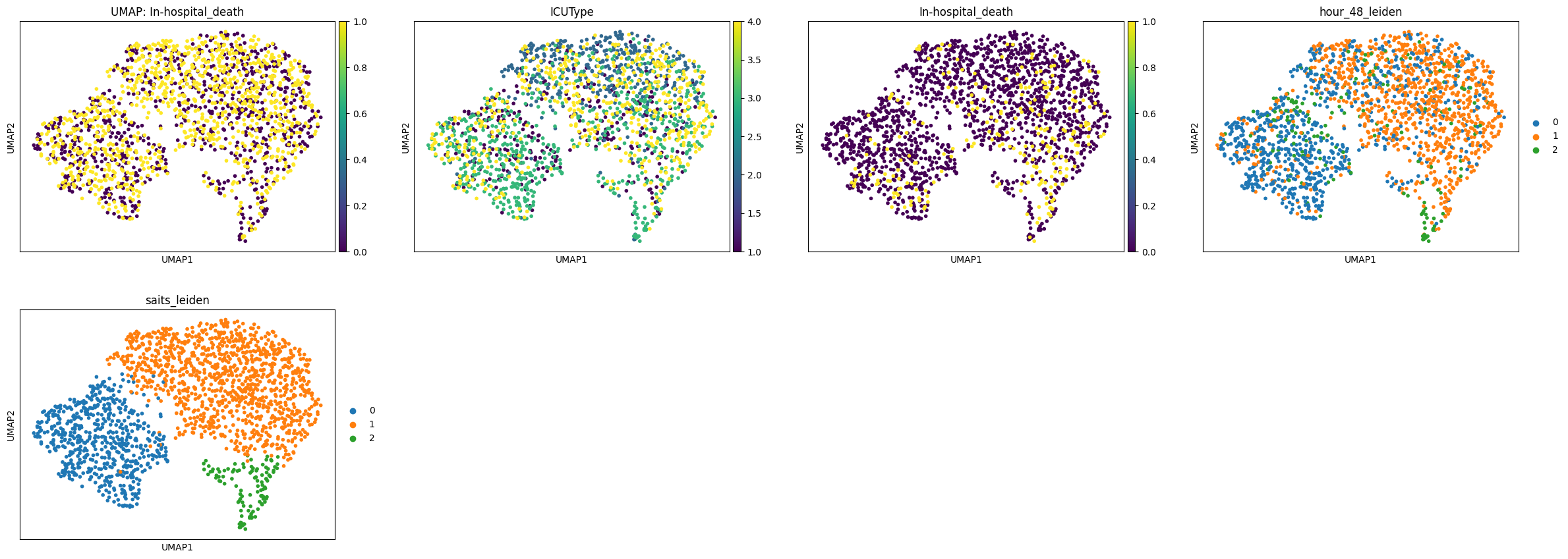
We don’t see clear cues from the static variables with the time-series information generated embedding. We can as before again compare the Leiden cluster’s based on e.g. their static information:

ep.tl.rank_features_groups(
    edata_test,
    field_to_rank="obs",
    columns_to_rank={"obs_names": ["Age", "Gender", "SAPS-I", "SOFA", "Length_of_stay", "missing_values_pct"]},
    groupby="saits_leiden",
    key_added="rank_features_groups",
)
ep.pl.rank_features_groups(edata_test, key="rank_features_groups", n_features=10, show=False)

! Feature  was detected as categorical features stored numerically.Please verify and correct using `ep.ad.replace_feature_types` if necessary.

! Detected no columns that need to be encoded. Leaving passed EHRData/AnnData object unchanged.

[<Axes: title={'center': '0 vs. rest'}, xlabel='ranking', ylabel='score'>,
 <Axes: title={'center': '1 vs. rest'}, xlabel='ranking'>,
 <Axes: title={'center': '2 vs. rest'}, xlabel='ranking'>]

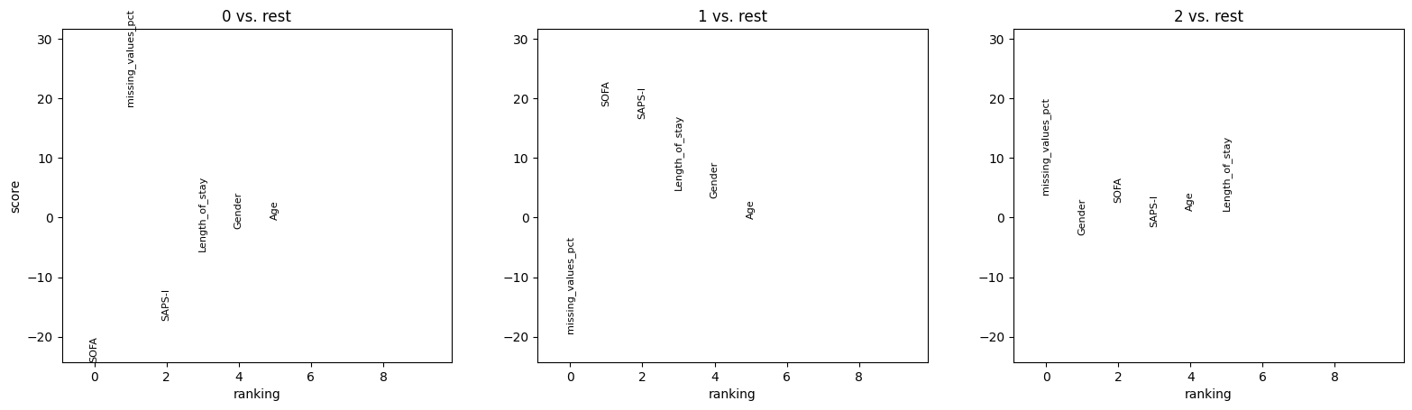
We can find again that clusters are corresponding to particularly high (and low) fractions of missing values, and low vs high SOFA and SAPS-I scores.

Cohort Tracking Summary

Let’s visualize how our cohort changed throughout the analysis pipeline.

ct.plot_cohort_barplot(subfigure_title=True, show=True, fontsize=9)

ct.plot_flowchart(title="Data Processing Pipeline Flowchart", show=True)

This concludes our walk-through of exploring this clinical longitudinal dataset and training a deep-learning classifier for predicting in-hospital mortality.

Resources

• PhysioNet 2012 Challenge: https://physionet.org/content/challenge-2012/1.0.0/

• RAINDROP & other classifiers in PyPOTS: https://docs.pypots.com/en/latest/pypots.classification.html

• PyPOTS: https://github.com/WenjieDu/PyPOTS

• ehrapy Documentation: https://ehrapy.readthedocs.io/

• ehrdata Documentation: https://ehrdata.readthedocs.io/