Note
This page was generated from mimic_2_causal_inference.ipynb. Some tutorial content may look better in light mode.
MIMIC-II IAC Causal Inference
This tutorial continues the exploration the MIMIC-II IAC dataset using causal inference methods. The dataset was created for the purpose of a case study in the book: Secondary Analysis of Electronic Health Records, published by Springer in 2016. In particular, the dataset was used throughout Chapter 16 (Data Analysis) by Raffa J. et al. to investigate the effectiveness of indwelling arterial catheters in hemodynamically stable patients with respiratory failure for mortality outcomes. The dataset is derived from MIMIC-II, the publicly-accessible critical care database. It contains summary clinical data and outcomes for 1,776 patients.
Reference:
[1] https://github.com/py-why/dowhy
[2] https://www.pywhy.org/dowhy/
[3] https://arxiv.org/abs/2011.04216
[4] https://physionet.org/content/mimic2-iaccd/1.0/
Importing ehrapy and setting plotting parameters
[1]:
import ehrapy as ep
from IPython.display import display
import graphviz
[2]:
import warnings

warnings.filterwarnings("ignore")
[3]:
ep.print_versions()
-----
ehrapy              0.9.0
rich                NA
scanpy              1.9.3
session_info        1.0.0
-----
CoreFoundation              NA
Foundation                  NA
Levenshtein                 0.21.1
PIL                         10.0.0
PyObjCTools                 NA
anndata                     0.9.2
anyio                       NA
appnope                     0.1.3
argcomplete                 NA
arrow                       1.2.3
astor                       0.8.1
asttokens                   NA
attr                        23.1.0
attrs                       23.1.0
autograd                    NA
autograd_gamma              NA
babel                       2.12.1
backcall                    0.2.0
brotli                      1.0.9
cachetools                  5.3.1
causallearn                 NA
certifi                     2023.07.22
cffi                        1.15.1
charset_normalizer          3.2.0
cloudpickle                 2.2.1
comm                        0.1.3
cvxopt                      1.3.1
cycler                      0.10.0
cython_runtime              NA
dateutil                    2.8.2
db_dtypes                   1.1.1
debugpy                     1.6.7
decorator                   5.1.1
defusedxml                  0.7.1
dill                        0.3.7
dot_parser                  NA
dowhy                       0.11.1
executing                   1.2.0
fastjsonschema              NA
fhiry                       3.0.0
filelock                    3.12.2
formulaic                   0.6.4
fqdn                        NA
future                      0.18.3
gmpy2                       2.1.2
google                      NA
graphlib                    NA
graphviz                    0.20.1
grpc                        1.56.2
grpc_status                 NA
h5py                        3.9.0
idna                        3.4
igraph                      0.10.6
imblearn                    0.12.3
interface_meta              1.3.0
ipykernel                   6.25.0
ipywidgets                  8.0.7
isoduration                 NA
jedi                        0.19.0
jinja2                      3.1.4
joblib                      1.3.0
json5                       NA
jsonpointer                 2.0
jsonschema                  4.18.4
jsonschema_specifications   NA
jupyter_events              0.7.0
jupyter_server              2.7.0
jupyterlab_server           2.24.0
kiwisolver                  1.4.4
lamin_utils                 0.13.2
leidenalg                   0.10.1
lifelines                   0.27.7
llvmlite                    0.40.1
markupsafe                  2.1.3
matplotlib                  3.7.2
missingno                   0.5.2
mpl_toolkits                NA
mpmath                      1.3.0
natsort                     8.4.0
nbformat                    5.9.2
networkx                    3.1
numba                       0.57.1
numpy                       1.24.0
objc                        9.2
overrides                   NA
packaging                   23.1
pandas                      2.0.3
parso                       0.8.3
patsy                       0.5.6
pexpect                     4.8.0
pickleshare                 0.7.5
pkg_resources               NA
platformdirs                3.10.0
prometheus_client           NA
prompt_toolkit              3.0.39
psutil                      5.9.5
ptyprocess                  0.7.0
pure_eval                   0.2.2
pyarrow                     12.0.1
pyasn1                      0.5.0
pyasn1_modules              0.3.0
pydev_ipython               NA
pydevconsole                NA
pydevd                      2.9.5
pydevd_file_utils           NA
pydevd_plugins              NA
pydevd_tracing              NA
pydot                       1.4.2
pygments                    2.15.1
pyparsing                   3.0.9
pythonjsonlogger            NA
pytz                        2023.3
rapidfuzz                   3.1.2
referencing                 NA
requests                    2.31.0
rfc3339_validator           0.1.4
rfc3986_validator           0.1.1
rpds                        NA
rsa                         4.9
scipy                       1.11.1
seaborn                     0.12.2
send2trash                  NA
setuptools                  68.0.0
six                         1.16.0
sklearn                     1.3.0
sniffio                     1.3.0
socks                       1.7.1
sphinxcontrib               NA
stack_data                  0.6.2
statsmodels                 0.14.2
sympy                       1.12
tableone                    0.9.1
tabulate                    0.9.0
texttable                   1.6.7
thefuzz                     0.19.0
threadpoolctl               3.2.0
torch                       2.0.1
tornado                     6.3.2
tqdm                        4.65.0
traitlets                   5.9.0
typing_extensions           NA
uri_template                NA
urllib3                     2.0.4
vscode                      NA
wcwidth                     0.2.6
webcolors                   1.13
websocket                   1.6.1
wrapt                       1.15.0
yaml                        6.0
zmq                         25.1.0
zoneinfo                    NA
-----
IPython             8.14.0
jupyter_client      8.3.0
jupyter_core        5.3.1
jupyterlab          4.0.3
notebook            7.0.1
-----
Python 3.10.12 | packaged by conda-forge | (main, Jun 23 2023, 22:41:52) [Clang 15.0.7 ]
macOS-13.1-arm64-arm-64bit
-----
Session information updated at 2024-06-28 11:35
MIMIC-II dataset preparation
Let’s load the MIMIC-II dataset using ehrapy with default one-hot encoding.
[4]:
adata = ep.dt.mimic_2(encoded=True)
The MIMIC-II dataset has 1776 patients as described above with 46 features.
[5]:
adata
[5]:
AnnData object with n_obs × n_vars = 1776 × 54
    obs: 'service_unit', 'day_icu_intime'
    var: 'feature_type', 'unencoded_var_names', 'encoding_mode'
    layers: 'original'
Causal Inference on the MIMIC-II dataset
In the background, ehrapy uses the dowhy package to enable effortless causal inference on electronic health records (EHR). Any dowhy analysis is structured into 3 steps: 1) Formulate causal questions 2) Estimate causal effects 3) Perform refutation tests.
Within ehrapy, we have consolidated this method into a single function ehrapy.causal_inference(). This function takes in the dataset, the treatment variable, the outcome variable, and the further optional parameters. It then performs the 3 steps above and displays the information in a user-friendly way.
Causal Graph
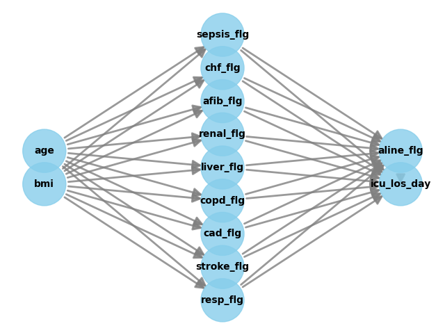
The causal graph is a directed acyclic graph (DAG) that represents the causal relationships between the variables in the dataset. Here, we create it by manually writing out the connections between the variables. Other options would be the GML or DOT graph format. Furthermore, you can use graphical tools like DAGitty to construct the graph. You can export the graph string that it generates. The graph string is very close to the DOT format: just rename dag to digraph, remove newlines and add a semicolon after every line, to convert it to the DOT format and input to DoWhy.
Assumptions:
both age and overweight increase your risk for medical problems
having a lot of problems makes you more likely to die in the hospital
having a lot of problems influences your likelihood of getting an IAC
having an IAC influences your likelihood of dying in the hospital
[6]:
causal_graph = """digraph {
aline_flg[label="Indwelling arterial catheters used"];
icu_los_day[label="Days in ICU"];

age -> sepsis_flg;
age -> chf_flg;
age -> afib_flg;
age -> renal_flg;
age -> liver_flg;
age -> copd_flg;
age -> cad_flg;
age -> stroke_flg;
age -> resp_flg;
bmi -> sepsis_flg;
bmi -> chf_flg;
bmi -> afib_flg;
bmi -> renal_flg;
bmi -> liver_flg;
bmi -> copd_flg;
bmi -> cad_flg;
bmi -> stroke_flg;
bmi -> resp_flg;
sepsis_flg -> aline_flg;
chf_flg -> aline_flg;
afib_flg -> aline_flg;
renal_flg -> aline_flg;
liver_flg -> aline_flg;
copd_flg -> aline_flg;
cad_flg -> aline_flg;
stroke_flg -> aline_flg;
resp_flg -> aline_flg;
sepsis_flg -> icu_los_day;
chf_flg -> icu_los_day;
afib_flg -> icu_los_day;
renal_flg -> icu_los_day;
liver_flg -> icu_los_day;
copd_flg -> icu_los_day;
cad_flg -> icu_los_day;
stroke_flg -> icu_los_day;
resp_flg -> icu_los_day;
aline_flg -> icu_los_day;
}"""

g = graphviz.Source(causal_graph)
display(g)

Causal inference
This graph can now be fed into the causal_inference() method. Furthermore, we have to specify an estimation_method. For now, we will use backdoor.linear_regression. Please refer to this example notebook and the official dowhy documentation for more information on the different estimation methods.
[7]:
ep.tl.causal_inference(
    adata=adata,
    graph=causal_graph,
    treatment="aline_flg",
    outcome="icu_los_day",
    estimation_method="backdoor.linear_regression",
)
❗ Refutation 'placebo_treatment_refuter' returned invalid pval 'nan', retrying (1/10)
❗ Refutation 'placebo_treatment_refuter' returned invalid pval 'nan', retrying (2/10)
❗ Refutation 'placebo_treatment_refuter' returned invalid pval 'nan', retrying (3/10)
❗ Refutation 'placebo_treatment_refuter' returned invalid pval 'nan', retrying (4/10)
❗ Refutation 'placebo_treatment_refuter' returned invalid pval 'nan', retrying (5/10)
❗ Refutation 'placebo_treatment_refuter' returned invalid pval 'nan', retrying (6/10)
❗ Refutation 'placebo_treatment_refuter' returned invalid pval 'nan', retrying (7/10)
❗ Refutation 'placebo_treatment_refuter' returned invalid pval 'nan', retrying (8/10)
❗ Refutation 'placebo_treatment_refuter' returned invalid pval 'nan', retrying (9/10)
❗ Refutation 'placebo_treatment_refuter' returned invalid pval 'nan', retrying (10/10)
Causal inference results for treatment variable 'aline_flg' and outcome variable 'icu_los_day':
└- Increasing the treatment variable(s) [aline_flg] from 0 to 1 causes an increase of 2.2348813091683186 in the expected value of the outcome [['icu_los_day']], over the data distribution/population represented by the dataset.
Refutation results
├-Refute: Use a Placebo Treatment
| ├- Estimated effect: 2.23
| ├- New effect: 0.000
| ├- p-value: nan
| └- Test significance: 2.23
├-Refute: Add a random common cause
| ├- Estimated effect: 2.23
| ├- New effect: 2.235
| ├- p-value: 0.494
| └- Test significance: 2.23
├-Refute: Use a subset of data
| ├- Estimated effect: 2.23
| ├- New effect: 2.233
| ├- p-value: 0.489
| └- Test significance: 2.23
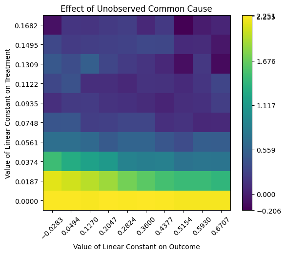
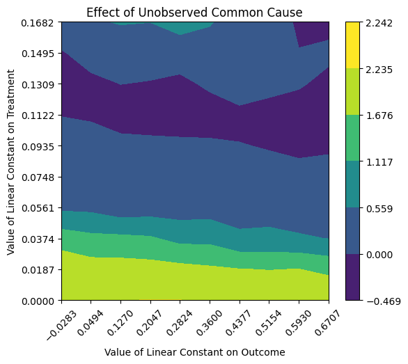
├-Refute: Add an Unobserved Common Cause
| ├- Estimated effect: 2.23
| ├- New effect: -0.25, 2.27
| ├- p-value: Not applicable
| └- Test significance: 2.23
├-Refute: Bootstrap Sample Dataset
| ├- Estimated effect: 2.23
| ├- New effect: 2.253
| ├- p-value: 0.453
| └- Test significance: 2.23
└-Refute: Use a Dummy Outcome
├- Estimated effect: 0.00
├- New effect: -0.008
├- p-value: 0.436
└- Test significance: 0.00
As we can see, the model returns a summary of the identified causal effect and the refutation results. The placebo_treatment_refuter failed in this case because our intervention variable is binary. By default, all 6 potential refutation methods are run, but the user can also specify to only use a subset of them.
[8]:
ep.tl.causal_inference(
    adata=adata,
    graph=causal_graph,
    treatment="aline_flg",
    outcome="icu_los_day",
    estimation_method="backdoor.linear_regression",
    refute_methods=[
        "placebo_treatment_refuter",
        "random_common_cause",
        "data_subset_refuter",
        "add_unobserved_common_cause",
        "bootstrap_refuter",
        "dummy_outcome_refuter",
    ],
)
❗ Refutation 'placebo_treatment_refuter' returned invalid pval 'nan', retrying (1/10)
❗ Refutation 'placebo_treatment_refuter' returned invalid pval 'nan', retrying (2/10)
❗ Refutation 'placebo_treatment_refuter' returned invalid pval 'nan', retrying (3/10)
❗ Refutation 'placebo_treatment_refuter' returned invalid pval 'nan', retrying (4/10)
❗ Refutation 'placebo_treatment_refuter' returned invalid pval 'nan', retrying (5/10)
❗ Refutation 'placebo_treatment_refuter' returned invalid pval 'nan', retrying (6/10)
❗ Refutation 'placebo_treatment_refuter' returned invalid pval 'nan', retrying (7/10)
❗ Refutation 'placebo_treatment_refuter' returned invalid pval 'nan', retrying (8/10)
❗ Refutation 'placebo_treatment_refuter' returned invalid pval 'nan', retrying (9/10)
❗ Refutation 'placebo_treatment_refuter' returned invalid pval 'nan', retrying (10/10)
Causal inference results for treatment variable 'aline_flg' and outcome variable 'icu_los_day':
└- Increasing the treatment variable(s) [aline_flg] from 0 to 1 causes an increase of 2.2348813091683186 in the expected value of the outcome [['icu_los_day']], over the data distribution/population represented by the dataset.

Refutation results
├-Refute: Use a Placebo Treatment
|    ├- Estimated effect: 2.23
|    ├- New effect: 0.000
|    ├- p-value: nan
|    └- Test significance: 2.23
├-Refute: Add a random common cause
|    ├- Estimated effect: 2.23
|    ├- New effect: 2.234
|    ├- p-value: 0.441
|    └- Test significance: 2.23
├-Refute: Use a subset of data
|    ├- Estimated effect: 2.23
|    ├- New effect: 2.243
|    ├- p-value: 0.447
|    └- Test significance: 2.23
├-Refute: Add an Unobserved Common Cause
|    ├- Estimated effect: 2.23
|    ├- New effect: -0.6, 2.25
|    ├- p-value: Not applicable
|    └- Test significance: 2.23
├-Refute: Bootstrap Sample Dataset
|    ├- Estimated effect: 2.23
|    ├- New effect: 2.219
|    ├- p-value: 0.454
|    └- Test significance: 2.23
└-Refute: Use a Dummy Outcome
     ├- Estimated effect: 0.00
     ├- New effect: 0.007
     ├- p-value: 0.437
     └- Test significance: 0.00
By default, we are hiding a lot of the default dowhy output for clarity. However, it is possible to nontheless display it.
[9]:
ep.tl.causal_inference(
    adata=adata,
    graph=causal_graph,
    treatment="aline_flg",
    outcome="icu_los_day",
    estimation_method="backdoor.linear_regression",
    refute_methods=[
        # "placebo_treatment_refuter",  # we know it'll fail
        "random_common_cause",
        "data_subset_refuter",
        "add_unobserved_common_cause",
        "bootstrap_refuter",
        "dummy_outcome_refuter",
    ],
    print_causal_estimate=True,
    print_summary=False,
)
*** Causal Estimate ***

## Identified estimand
Estimand type: EstimandType.NONPARAMETRIC_ATE

### Estimand : 1
Estimand name: backdoor
Estimand expression:
     d
────────────(E[icu_los_day|stroke_flg,copd_flg,sepsis_flg,liver_flg,resp_flg,c
d[aline_flg]


ad_flg,chf_flg,renal_flg,afib_flg])

Estimand assumption 1, Unconfoundedness: If U→{aline_flg} and U→icu_los_day then P(icu_los_day|aline_flg,stroke_flg,copd_flg,sepsis_flg,liver_flg,resp_flg,cad_flg,chf_flg,renal_flg,afib_flg,U) = P(icu_los_day|aline_flg,stroke_flg,copd_flg,sepsis_flg,liver_flg,resp_flg,cad_flg,chf_flg,renal_flg,afib_flg)

## Realized estimand
b: icu_los_day~aline_flg+stroke_flg+copd_flg+sepsis_flg+liver_flg+resp_flg+cad_flg+chf_flg+renal_flg+afib_flg
Target units: ate

## Estimate
Mean value: 2.2348813091683186
Plotting
Furthermore, the causal_inference() function can generate several plots, if desired. It’s for example possible to output the causal graph …
[10]:
ep.tl.causal_inference(
    adata=adata,
    graph=causal_graph,
    treatment="aline_flg",
    outcome="icu_los_day",
    estimation_method="backdoor.linear_regression",
    refute_methods=[
        # "placebo_treatment_refuter",  # we know it'll fail
        "random_common_cause",
        "data_subset_refuter",
        "add_unobserved_common_cause",
        "dummy_outcome_refuter",
    ],
    print_causal_estimate=False,
    print_summary=False,
    show_graph=True,
)
… or the graph generated by the add_unobserved_common_cause refutation method.
[11]:
ep.tl.causal_inference(
    adata=adata,
    graph=causal_graph,
    treatment="aline_flg",
    outcome="icu_los_day",
    estimation_method="backdoor.linear_regression",
    refute_methods=[
        # "placebo_treatment_refuter",  # we know it'll fail
        "random_common_cause",
        "data_subset_refuter",
        "add_unobserved_common_cause",
        "dummy_outcome_refuter",
    ],
    print_causal_estimate=False,
    print_summary=False,
    show_graph=False,
    show_refute_plots=True,
)
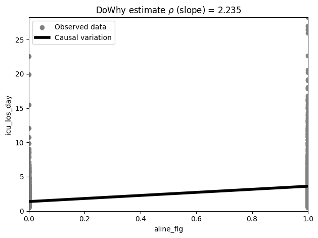
In the process of performing the causal dowhy analysis, an estimator is created which we can query from the model and then visualise.
[12]:
estimate = ep.tl.causal_inference(
    adata=adata,
    graph=causal_graph,
    treatment="aline_flg",
    outcome="icu_los_day",
    estimation_method="backdoor.linear_regression",
    refute_methods=[
        # "placebo_treatment_refuter",  # we know it'll fail
        "random_common_cause",
        "data_subset_refuter",
        "add_unobserved_common_cause",
        "bootstrap_refuter",
        "dummy_outcome_refuter",
    ],
    print_causal_estimate=False,
    print_summary=False,
    show_graph=False,
    show_refute_plots=False,
    return_as="estimate",
)
[13]:
ep.pl.causal_effect(estimate)
[13]:
<Axes: title={'center': 'DoWhy estimate $\\rho$ (slope) = 2.235'}, xlabel='aline_flg', ylabel='icu_los_day'>
Advanced options
Within dowhy, the user can specify several arguments for identification, estimation and refutation. These arguments can also be passed directly to the respective functions through the identify_kwargs, estimate_kwargs and refute_kwarg of causal_inference().
[14]:
estimate = ep.tl.causal_inference(
    adata=adata,
    graph=causal_graph,
    treatment="aline_flg",
    outcome="icu_los_day",
    estimation_method="backdoor.linear_regression",
    refute_methods=[
        # "placebo_treatment_refuter",  # we know it'll fail
        "random_common_cause",
        "data_subset_refuter",
        "add_unobserved_common_cause",
        "bootstrap_refuter",
        "dummy_outcome_refuter",
    ],
    print_causal_estimate=True,
    print_summary=True,
    show_graph=False,
    show_refute_plots="contour",
    return_as="estimate",
    identify_kwargs={"proceed_when_unidentifiable": True},
    estimate_kwargs={"target_units": "days"},
    refute_kwargs={"random_seed": 5},
)
*** Causal Estimate ***

## Identified estimand
Estimand type: EstimandType.NONPARAMETRIC_ATE

### Estimand : 1
Estimand name: backdoor
Estimand expression:
     d
────────────(E[icu_los_day|stroke_flg,copd_flg,sepsis_flg,liver_flg,resp_flg,c
d[aline_flg]


ad_flg,chf_flg,renal_flg,afib_flg])

Estimand assumption 1, Unconfoundedness: If U→{aline_flg} and U→icu_los_day then P(icu_los_day|aline_flg,stroke_flg,copd_flg,sepsis_flg,liver_flg,resp_flg,cad_flg,chf_flg,renal_flg,afib_flg,U) = P(icu_los_day|aline_flg,stroke_flg,copd_flg,sepsis_flg,liver_flg,resp_flg,cad_flg,chf_flg,renal_flg,afib_flg)

## Realized estimand
b: icu_los_day~aline_flg+stroke_flg+copd_flg+sepsis_flg+liver_flg+resp_flg+cad_flg+chf_flg+renal_flg+afib_flg
Target units: days

## Estimate
Mean value: 2.2348813091683186

Causal inference results for treatment variable 'aline_flg' and outcome variable 'icu_los_day':
└- Increasing the treatment variable(s) [aline_flg] from 0 to 1 causes an increase of 2.2348813091683186 in the expected value of the outcome [['icu_los_day']], over the data distribution/population represented by the dataset.

Refutation results
├-Refute: Add a random common cause
|    ├- Estimated effect: 2.23
|    ├- New effect: 2.234
|    ├- p-value: 0.399
|    └- Test significance: 2.23
├-Refute: Use a subset of data
|    ├- Estimated effect: 2.23
|    ├- New effect: 2.228
|    ├- p-value: 0.464
|    └- Test significance: 2.23
├-Refute: Add an Unobserved Common Cause
|    ├- Estimated effect: 2.23
|    ├- New effect: -0.47, 2.24
|    ├- p-value: Not applicable
|    └- Test significance: 2.23
├-Refute: Bootstrap Sample Dataset
|    ├- Estimated effect: 2.23
|    ├- New effect: 2.240
|    ├- p-value: 0.482
|    └- Test significance: 2.23
└-Refute: Use a Dummy Outcome
     ├- Estimated effect: 0.00
     ├- New effect: 0.008
     ├- p-value: 0.441
     └- Test significance: 0.00